/*! This file is auto-generated */ .wp-block-button__link{color:#fff;background-color:#32373c;border-radius:9999px;box-shadow:none;text-decoration:none;padding:calc(.667em + 2px) calc(1.333em + 2px);font-size:1.125em}.wp-block-file__button{background:#32373c;color:#fff;text-decoration:none} Q5E As an example of a situation in ... [FREE SOLUTION] | 魅影直播

魅影直播

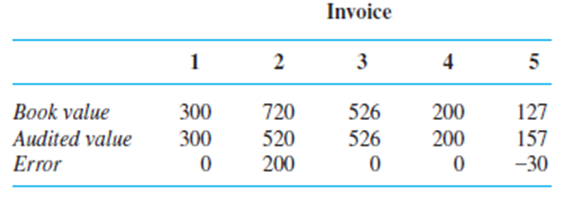
As an example of a situation in which several different statis tics could reasonably be used to calculate a point estimate, consider a population of N invoices. Associated with each invoice is its 鈥渂ook value,鈥 the recorded amount of that invoice. Let T denote the total book value, a known amount. Some of these book values are erroneous. An audit will be carried out by randomly selecting n invoices and determining the audited (correct) value for each one. Suppose that the sample gives the following
\({\rm{T}}\)- sample mean book value

\(\bar X\)- sample mean advised value

\({\rm{\bar D}}\)- sample mean errors

Propose three different statistics for estimating the total audited (i.e., correct) value-one involving just N and,another involving T, N, and \({\rm{\bar D,}}\) and the last involving T and \({\rm{\bar X/\bar Y}}{\rm{.}}\)If \({\rm{N = 5000}}\)and T=1,761,300, calculate the three corresponding point estimates. (The article "Statistical Models and Analysis in Auditing," Statistical Science, 1989: 2-33 discusses properties of these estimators.)

Short Answer

Expert verified

a.The estimated value is\({\rm{1,704,000}}\).

b.The estimated value is\({\rm{1,591,300}}\).

c.The estimated value is\({\rm{1,601,438}}{\rm{.281}}\).

Step by step solution

01

Concept introduction

The standard deviation (SD) is a measure of the variability, or dispersion, between individual data values and the mean, whereas the standard error of the mean (SEM) is a measure of how far the sample mean (average) of the data is expected to differ from the genuine population mean. Always, the SEM is smaller than the SD.

02

Calculating the total audited values

The total audited values are denoted by\({\theta _T}\).

First, using simply\(N\)and\(\bar X\)the following statistic can be employed.

\({{\rm{\hat \theta }}_{{{\rm{T}}_{\rm{1}}}}}{\rm{ = N \times \bar X}}\)

Which is simply the \(N\) invoice multiplied by the average.

Second, using\({\rm{N \times \bar X}}\), and\(\bar D\), the following statistic can be employed.

\({{\rm{\hat \theta }}_{{{\rm{T}}_{\rm{2}}}}}{\rm{ = T - N \times \bar D}}\)

When the total sample mean error is deducted from the total book value, the total book value is the result.

Third, using \(T\)and \(\bar X/\bar Y\),the following statistic can be employed.

This is the quotient of the sample mean audited value and the sample mean book average multiplied by the total book value: \({{\rm{\hat \theta }}_{{{\rm{T}}_{\rm{3}}}}}{\rm{ = T \times }}\frac{{{\rm{\bar X}}}}{{{\rm{\bar Y}}}}\)

03

Estimating the point using the invoice table

Consider the given,

\(\begin{array}{l}{\rm{N = 5000 }}\\{\rm{T = 1,761,300}}\end{array}\)

The point estimations can be determined using the invoice table and the invoice table

\(\begin{array}{c}{\rm{\bar y = }}\frac{{\rm{1}}}{{\rm{5}}}{\rm{(300 + 720 + 526 + 200 + 127)}}\\{\rm{ = 374}}{\rm{.6}}\end{array}\)

The average audited value in the sample is

\(\begin{array}{c}{\rm{\bar x = }}\frac{{\rm{1}}}{{\rm{5}}}{\rm{(300 + 520 + 526 + 200 + 157)}}\\{\rm{ = 340}}{\rm{.6,}}\end{array}\)

Where the standard deviation of the sample mean error is

\(\begin{array}{c}{\rm{\bar d = }}\frac{{\rm{1}}}{{\rm{5}}}{\rm{(0 + 200 + 0 + 0 - 30)}}\\{\rm{ = 34}}\end{array}\)

As a result, the point estimations

\(\begin{array}{c}{\rm{\& }}{{{\rm{\hat \theta }}}_{{{\rm{T}}_{\rm{1}}}}}{\rm{ = N \times \bar x = 5000 \times 340}}{\rm{.6}}\\{\rm{ = 1,704,000,}}\\{\rm{n\& }}{{{\rm{\hat \theta }}}_{{{\rm{T}}_{\rm{2}}}}}{\rm{ = T - N \times \bar d = 1,761,300 - 5,000 \times 34}}{\rm{.0}}\\{\rm{ = 1,591,300,}}\\{{{\rm{\hat \theta }}}_{{{\rm{T}}_{\rm{3}}}}}{\rm{ = T \times }}\frac{{{\rm{\bar x}}}}{{{\rm{\bar y}}}}\\{\rm{ = 1,761,300 \times }}\frac{{{\rm{340}}{\rm{.6}}}}{{{\rm{374}}{\rm{.6}}}}\\{\rm{ = 1,601,438}}{\rm{.281}}\end{array}\)

Therefore, the required estimated value is\({\rm{1,601,438}}{\rm{.281}}\).

Unlock Step-by-Step Solutions & Ace Your Exams!

  • Full Textbook Solutions

    Get detailed explanations and key concepts

  • Unlimited Al creation

    Al flashcards, explanations, exams and more...

  • Ads-free access

    To over 500 millions flashcards

  • Money-back guarantee

    We refund you if you fail your exam.

Over 30 million students worldwide already upgrade their learning with 魅影直播!

One App. One Place for Learning.

All the tools & learning materials you need for study success - in one app.

Get started for free

Most popular questions from this chapter

Fire load (MJ/m2) is the heat energy that could bereleased per square meter of floor area by combustionof contents and the structure itself. The article 鈥淔ireLoads in Office Buildings鈥 (J. of Structural Engr.,

1997: 365鈥368) gave the following cumulative percentages(read from a graph) for fire loads in a sample of388 rooms:

Value0 150 300 450 600

Cumulative %0 19.3 37.6 62.7 77.5

Value750 900 1050 1200 1350

Cumulative %87.2 93.8 95.7 98.6 99.1

Value1500 1650 1800 1950

Cumulative %99.5 99.6 99.8 100.0

a. Construct a relative frequency histogram and commenton interesting features.

b. What proportion of fire loads are less than 600? At least 1200?

c. What proportion of the loads are between 600 and1200?

The accompanying data set consists of observations on shear strength (lb) of ultrasonic spot welds made on a certain type of alclad sheet. Construct a relative frequency histogram based on ten equal-width classes with boundaries 4000, 4200, 鈥. [The histogram will agree with the one in 鈥淐omparison of Properties of Joints Prepared by Ultrasonic Welding and Other Means鈥 (J. of Aircraft, 1983: 552鈥556).] Comment on its features.

5434

4948

4521

4570

4990

5702

5241

5112

5015

4659

4806

4637

5670

4381

4820

5043

4886

4599

5288

5299

4848

5378

5260

5055

5828

5218

4859

4780

5027

5008

4609

4772

5133

5095

4618

4848

5089

5518

5333

5164

5342

5069

4755

4925

5001

4803

4951

5679

5256

5207

5621

4918

5138

4786

4500

5461

5049

4974

4592

4173

5296

4965

5170

4740

5173

4568

5653

5078

4900

4968

5248

5245

4723

5275

5419

5205

4452

5227

5555

5388

5498

4681

5076

4774

4931

4493

5309

5582

4308

4823

4417

5364

5640

5069

5188

5764

5273

5042

5189

4986

Consider the following sample of observations on coating thickness for low-viscosity paint ("Achieving a Target Value for a Manufacturing Process: \({\rm{A}}\)Case Study, \({\rm{97}}\)J. of Quality Technology, \({\rm{1992:22 - 26}}\)):

\(\begin{array}{*{20}{r}}{{\rm{.83}}}&{{\rm{.88}}}&{{\rm{.88}}}&{{\rm{1}}{\rm{.04}}}&{{\rm{1}}{\rm{.09}}}&{{\rm{1}}{\rm{.12}}}&{{\rm{1}}{\rm{.29}}}&{{\rm{1}}{\rm{.31}}}\\{{\rm{1}}{\rm{.48}}}&{{\rm{1}}{\rm{.49}}}&{{\rm{1}}{\rm{.59}}}&{{\rm{1}}{\rm{.62}}}&{{\rm{1}}{\rm{.65}}}&{{\rm{1}}{\rm{.71}}}&{{\rm{1}}{\rm{.76}}}&{{\rm{1}}{\rm{.83}}}\end{array}\)

Assume that the distribution of counting thickness is normal (a normal probability plot strongly supports this assumption).

a. Calculate a point estimate of the mean value of coating thickness, and state which estimator you used.

b. Calculate a point estimate of the median of the coating thickness distribution, and state which estimator you used.

C. Calculate a point estimate of the value that separates the largest of\({\rm{10\% }}\) all values in the thickness distribution from the remaining \({\rm{90\% }}\)and state which estimator you used. (Hint Express what you are trying to estimate in terms of \({\rm{\mu }}\)and \({\rm{\sigma }}\)

d. Estimate \({\rm{P}}\left( {{\rm{X < 1}}{\rm{.5}}} \right){\rm{,}}\)i.e., the proportion of all thickness values less than 1.5. (Hint: If you knew the values of \({\rm{\mu }}\)and \({\rm{\sigma }}\), you could calculate this probability. These values are not available, but they can be estimated.)

e. What is the estimated standard error of the estimator that you used in part (b)?

Exposure to microbial products, especially endotoxin, may have an impact on vulnerability to allergic diseases. The article 鈥淒ust Sampling Methods for Endotoxin鈥擜n Essential, But Underestimated Issue鈥 (Indoor Air,2006: 20鈥27) considered various issues associated with determining endotoxin concentration. The following data on concentration (EU/mg) in settled dust for one sample of urban homes and another of farm homes was kindly supplied by the authors of the cited article.

U: 6.0 5.0 11.0 33.0 4.0 5.0 80.0 18.0 35.0 17.0 23.0

F: 4.0 14.0 11.0 9.0 9.0 8.0 4.0 20.0 5.0 8.9 21.0

9.2 3.0 2.0 0.3

  1. Determine the sample mean for each sample. How do they compare?
  2. Determine the sample median for each sample. How do they compare? Why is the median for the urban sample so different from the mean for that sample?
  3. Calculate the trimmed mean for each sample by deleting the smallest and largest observation. What are the corresponding trimming percentages? How do the values of these trimmed means compare to the corresponding means and medians?

A Pareto diagram is a variation of a histogram forcategorical data resulting from a quality control study.Each category represents a different type of product non-conformity or production problem. The categories areordered so that the one with the largest frequencyappears on the far left, then the category with the secondlargest frequency, and so on. Suppose the following information on nonconformities in circuit packs isobtained: failed component, 126; incorrect component,210; insufficient solder, 67; excess solder, 54; missingcomponent, 131. Construct a Pareto diagram.

See all solutions

Recommended explanations on Math Textbooks

View all explanations

What do you think about this solution?

We value your feedback to improve our textbook solutions.

Study anywhere. Anytime. Across all devices.
