/*! This file is auto-generated */ .wp-block-button__link{color:#fff;background-color:#32373c;border-radius:9999px;box-shadow:none;text-decoration:none;padding:calc(.667em + 2px) calc(1.333em + 2px);font-size:1.125em}.wp-block-file__button{background:#32373c;color:#fff;text-decoration:none} Q34E Exposure to microbial products, ... [FREE SOLUTION] | 魅影直播

魅影直播

Exposure to microbial products, especially endotoxin, may have an impact on vulnerability to allergic diseases. The article 鈥淒ust Sampling Methods for Endotoxin鈥擜n Essential, But Underestimated Issue鈥 (Indoor Air,2006: 20鈥27) considered various issues associated with determining endotoxin concentration. The following data on concentration (EU/mg) in settled dust for one sample of urban homes and another of farm homes was kindly supplied by the authors of the cited article.

U: 6.0 5.0 11.0 33.0 4.0 5.0 80.0 18.0 35.0 17.0 23.0

F: 4.0 14.0 11.0 9.0 9.0 8.0 4.0 20.0 5.0 8.9 21.0

9.2 3.0 2.0 0.3

  1. Determine the sample mean for each sample. How do they compare?
  2. Determine the sample median for each sample. How do they compare? Why is the median for the urban sample so different from the mean for that sample?
  3. Calculate the trimmed mean for each sample by deleting the smallest and largest observation. What are the corresponding trimming percentages? How do the values of these trimmed means compare to the corresponding means and medians?

Short Answer

Expert verified

a. The sample mean for one sample of urban homes is 21.5.The sample mean for farm homes is 8.6.

b. The sample median for one sample of urban homes is 17.The sample median for farm homes is 8.9.

c. The trimmed sample mean for urban homes is 17 and for another of farm homes is 8.24. The trimmed percentages for urban homes and farm homes are 9.09% and 6.67% respectively.

On comparison, trimmed mean is observed to be lower in magnitude than the corresponding mean and medians for each of the two variables.

Step by step solution

01

Given information

The data on the concentration (EU/mg) in settled dust for one sample of urban homes and another of farm homes are provided.

02

Compute the sample mean

Let x represents the concentration (EU/mg) in settled dust for one sample of urban homes.

Let y represent the concentration (EU/mg) in settled dust for another farm homes.

The sample mean is computed as,

For x,

\(\begin{array}{c}\bar x &=& \frac{{\sum {{x_i}} }}{n}\\ &=& \frac{{6 + 5 + 11 + ... + 23}}{{11}}\\ &=& \frac{{237}}{{11}}\\ &=& 21.5\end{array}\)

Thus, the sample mean for x is 21.5EU/mg.

For y,

\(\begin{array}{c}\bar y &=& \frac{{\sum {{y_i}} }}{{{n_y}}}\\ &=& \frac{{4 + 14 + 11 + ... + 0.3}}{{15}}\\ &=& \frac{{128.4}}{{15}}\\ &=& 8.6\end{array}\)

Thus, the sample mean for y is 8.6EU/mg.

Therefore, it can be concluded that the average concentration (EU/mg) in settled dust for one sample of urban homes is more than compared to the another of farm homes.

03

Compute the sample median

Let x represents the concentration (EU/mg) in settled dust for one sample of urban homes.

Let y represent the concentration (EU/mg) in settled dust for another farm homes.

The sample median is computed by first ordering the data in ascending order.

For x,

The data is arranged as,

4

5

5

6

11

17

18

23

33

35

80

For the odd number of observations, the median value is computed as,

\(\begin{array}{c}\tilde x &=& {\left( {\frac{{n + 1}}{2}} \right)^{th}}ordered\;value\\ &=& {\left( {\frac{{11 + 1}}{2}} \right)^{th}}ordered\;value\\ &=& {\left( 6 \right)^{th}}ordered\;value\end{array}\)

Thus, the median value of x is 17EU/mg.

For y,

The data is arranged as,

0.3

2

3

4

4

5

8

8.9

9

9

9.2

11

14

20

21

For the odd number of observations, the median value is computed as,

\(\begin{array}{c}\tilde y &=& {\left( {\frac{{n + 1}}{2}} \right)^{th}}ordered\;value\\ &=& {\left( {\frac{{15 + 1}}{2}} \right)^{th}}ordered\;value\\ &=& {\left( 8 \right)^{th}}ordered\;value\end{array}\)

Thus, the median value of y is 8.9EU/mg.

Therefore, it can be concluded that the median concentration (EU/mg) in settled dust for one sample of urban homes is more than compared to the another of farm homes.

The median for the urban sample is so different from the mean for that sample because mean represents the average and the median value represents the centre.

04

Compute the trimmed mean

Let x represents the concentration (EU/mg) in settled dust for one sample of urban homes.

Let y represent the concentration (EU/mg) in settled dust for another farm homes.

The trimmed mean for each sample is obtained by deleting few of the smallest and largest observation.

The trimmed data for x is,

5

5

6

11

17

18

23

33

35

The sample mean is computed as,

For x,

\(\begin{array}{c}{{\bar x}_{tr}} &=& \frac{{\sum {{x_i}} }}{n}\\ &=& \frac{{5 + 5 + 6 + ... + 35}}{9}\\ &=& \frac{{153}}{9}\\ &=& 17\end{array}\)

Thus, the trimmed mean for x is 17EU/mg.

The trimmed data for y is,

2

3

4

4

5

8

8.9

9

9

9.2

11

14

20

For y,

\(\begin{array}{c}{{\bar y}_{\left( {tr} \right)}} &=& \frac{{\sum {{y_i}} }}{{{n_y}}}\\ &=& \frac{{2 + 3 + 4 + ... + 20}}{{13}}\\ &=& \frac{{107.1}}{{13}}\\ &=& 8.2\end{array}\)

Thus, the trimmed mean for y is 8.2EU/mg.

05

Compute the trimmed percentages

The trimmed percentages (P) are computed using the following formula for each of the two samples.

\(\frac{P}{{100}}*N = K \Rightarrow {\bf{P = }}\frac{{\bf{K}}}{{\bf{N}}}*{\bf{100}}\)

Where N is the total number of observations and K is the number of values removed from each end.

In case of urban homes,

\(\begin{array}{l}N = 11\\K = 1\end{array}\)

The trimmed percentage is,

\(\begin{array}{c}{P_U} &=& \frac{1}{{11}}*100\\ &=& 9.09\% \end{array}\)

In case of farm homes,

\(\begin{array}{l}N = 15\\K = 1\end{array}\)

The trimmed percentage is,

\(\begin{array}{c}{P_F} &=& \frac{1}{{15}}*100\\ &=& 6.67\% \end{array}\)

On comparison of trimmed mean with the mean of the complete data, it is concluded that the trimmed mean is smaller in magnitude for both urban and farm homes.

Similarly, it is also observed that the trimmed mean is lower in magnitude than the median values.

Unlock Step-by-Step Solutions & Ace Your Exams!

  • Full Textbook Solutions

    Get detailed explanations and key concepts

  • Unlimited Al creation

    Al flashcards, explanations, exams and more...

  • Ads-free access

    To over 500 millions flashcards

  • Money-back guarantee

    We refund you if you fail your exam.

Over 30 million students worldwide already upgrade their learning with 魅影直播!

One App. One Place for Learning.

All the tools & learning materials you need for study success - in one app.

Get started for free

Most popular questions from this chapter

A sample of 77 individuals working at a particular office wasselected and the noise level (dBA) experienced by each individual was determined, yielding the followingdata (鈥淎cceptable Noise Levels for Construction Site Offices,鈥 Building Serv. Engr. Research and Technology, 2009: 87鈥94).

55.3

55.3

55.3

55.9

55.9

55.9

55.9

56.1

56.1

56.1

56.1

56.1

56.1

56.8

56.8

57.0

57.0

57.0

57.8

57.8

57.8

57.9

57.9

57.9

58.8

58.8

58.8

59.8

59.8

59.8

62.2

62.2

63.8

63.8

63.8

63.9

63.9

63.9

64.7

64.7

64.7

65.1

65.1

65.1

65.3

65.3

65.3

65.3

67.4

67.4

67.4

67.4

68.7

68.7

68.7

68.7

69.0

70.4

70.4

71.2

71.2

71.2

73.0

73.0

73.1

73.1

74.6

74.6

74.6

74.6

79.3

79.3

79.3

79.3

83.0

83.0

83.0

Use various techniques discussed in this chapter to organize, summarize, and describe the data.

The article 鈥淢onte Carlo Simulation鈥擳ool for Better Understanding of LRFD鈥 (J. of Structural Engr., \({\rm{1993: 1586 - 1599}}\)) suggests that yield strength (\({\rm{ksi}}\)) for A36 grade steel is normally distributed with \({\rm{\mu = 43}}\) and \({\rm{\sigma = 4}}{\rm{.5 }}\)

a. What is the probability that yield strength is at most \({\rm{40}}\)? Greater than \({\rm{60}}\)?

b. What yield strength value separates the strongest \({\rm{75\% }}\) from the others?

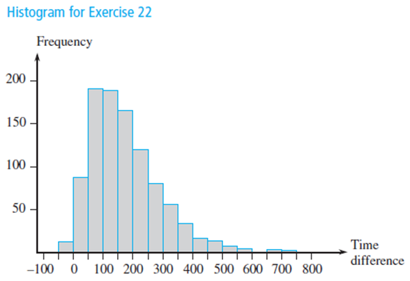
How does the speed of a runner vary over the course of a marathon (a distance of 42.195 km)? Consider determining both the time to run the first 5 km and the time to run between the 35-km and 40-km points, and then subtracting the former time from the latter time. A positive value of this difference corresponds to a runner slowing down toward the end of the race. The accompanying histogram is based on times of runners who participated in several different Japanese marathons (鈥淔actors Affecting Runners鈥 Marathon Performance,鈥 Chance, Fall, 1993: 24鈥30).What are some interesting features of this histogram? What is a typical difference value? Roughly what proportion of the runners ran the late distance more quickly than the early distance?

One piece of PVC pipe is to be inserted inside another piece. The length of the first piece is normally distributed with mean value \({\rm{20}}\) in. and standard deviation \({\rm{.5}}\) in. The length of the second piece is a normal \({\rm{rv}}\)with mean and standard deviation \({\rm{15}}\) in. and \({\rm{.4}}\) in., respectively. The amount of overlap is normally distributed with mean value \({\rm{1}}\) in. and standard deviation \({\rm{.1}}\) in. Assuming that the lengths and amount of overlap are independent of one another, what is the probability that the total length after insertion is between \({\rm{34}}{\rm{.5 }}\) in. and \({\rm{35}}\) in.?

The article 鈥淒etermination of Most RepresentativeSubdivision鈥 (J. of Energy Engr., 1993: 43鈥55) gavedata on various characteristics ofsubdivisions that couldbe used in deciding whether to provide electrical powerusing overhead lines or underground lines. Here are thevalues of the variable x=total length of streets within asubdivision:

1280

5320

4390

2100

1240

3060

4770

1050

360

3330

3380

340

1000

960

1320

530

3350

540

3870

1250

2400

960

1120

2120

450

2250

2320

2400

3150

5700

5220

500

1850

2460

5850

2700

2730

1670

100

5770

3150

1890

510

240

396

1419

2109

a. Construct a stem-and-leaf display using the thousandsdigit as the stem and the hundreds digit as theleaf, and comment on the various features of thedisplay.

b. Construct a histogram using class boundaries 0, 1000, 2000, 3000, 4000, 5000, and 6000. What proportion of subdivisions have a total length less than 2000? Between 2000 and 4000? How would you describe the shape of the histogram?

See all solutions

Recommended explanations on Math Textbooks

View all explanations

What do you think about this solution?

We value your feedback to improve our textbook solutions.

Study anywhere. Anytime. Across all devices.