Explanations
  Textbooks
  Flashcards
  魅影直播 AI
  Notes
Notes  Study Plans
  Study Sets
  Find a degree
  Magazine
 Chapter 1: Q63SE (page 47)
A sample of 77 individuals working at a particular office wasselected and the noise level (dBA) experienced by each individual was determined, yielding the followingdata (鈥淎cceptable Noise Levels for Construction Site Offices,鈥� Building Serv. Engr. Research and Technology, 2009: 87鈥�94).
55.3 | 55.3 | 55.3 | 55.9 | 55.9 | 55.9 | 55.9 | 56.1 | 56.1 | 56.1 | 56.1 |
56.1 | 56.1 | 56.8 | 56.8 | 57.0 | 57.0 | 57.0 | 57.8 | 57.8 | 57.8 | 57.9 |
57.9 | 57.9 | 58.8 | 58.8 | 58.8 | 59.8 | 59.8 | 59.8 | 62.2 | 62.2 | 63.8 |
63.8 | 63.8 | 63.9 | 63.9 | 63.9 | 64.7 | 64.7 | 64.7 | 65.1 | 65.1 | 65.1 |
65.3 | 65.3 | 65.3 | 65.3 | 67.4 | 67.4 | 67.4 | 67.4 | 68.7 | 68.7 | 68.7 |
68.7 | 69.0 | 70.4 | 70.4 | 71.2 | 71.2 | 71.2 | 73.0 | 73.0 | 73.1 | 73.1 |
74.6 | 74.6 | 74.6 | 74.6 | 79.3 | 79.3 | 79.3 | 79.3 | 83.0 | 83.0 | 83.0 |
Use various techniques discussed in this chapter to organize, summarize, and describe the data.
Short Answer
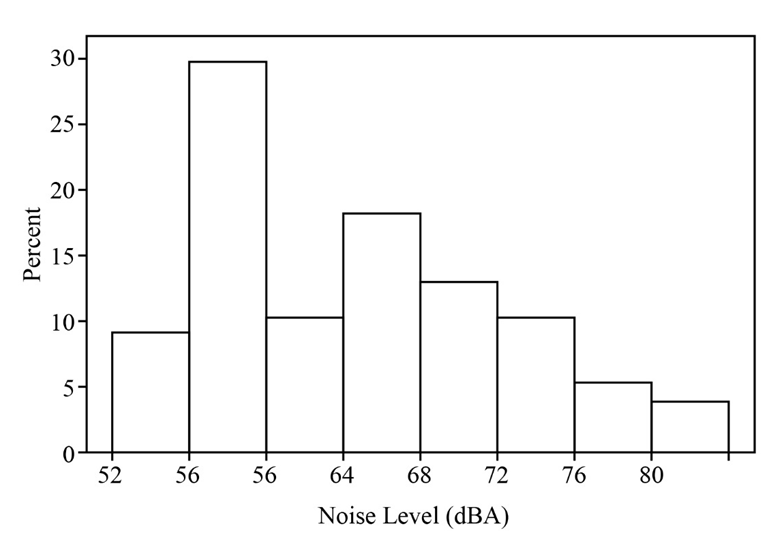
The histogram is nearly unimodal and most of the data values lies in the class interval of\(56 - < 60\).
The five-number summary are Smallest\({x_i}\): 55.3, lower fourth: 57.8, median: 64.7, upper fourth: 70.8, and largest\({x_i}\): 83.
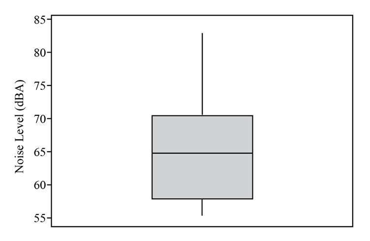
The boxplot shows that the data, is somewhat, negatively skewed. Because there are no outliers, there is less variation, and the upper whisker is larger than the lower one.
Step by step solution
Given information
The data are provided that consists of 77 observations on the noise level experienced by each individual.
Construct frequency distribution for the given data
The class width should be equal to 5. The following table shows three columns namely class, frequency and relative frequency:
Use this formula to calculate relative frequency of each data set,
\(relative{\rm{ }}frequency{\rm{ }}of{\rm{ }}a{\rm{ }}value = \frac{{number{\rm{ }}of{\rm{ }}times{\rm{ }}the{\rm{ }}value{\rm{ }}occurs}}{{number{\rm{ }}of{\rm{ }}observations{\rm{ }}in{\rm{ }}the{\rm{ }}data{\rm{ }}set}}\)
Class | Frequency | Relative Frequency |
52 - < 56 | 7 | \(0.0910\) |
56 - < 60 | 23 | 0.2987 |
60 - < 64 | 8 | 0.1039 |
64 - < 68 | 14 | 0.1818 |
68 - < 72 | 10 | 0.1299 |
72 - < 76 | 8 | 0.1039 |
76 - < 80 | 4 | 0.0519 |
80 - < 84 | 3 | 0.0390 |
Construct histogram using a frequency distribution table
Following are the steps to make a histogram:
1. On the vertical axis, place the frequencies and label this axis as 鈥淧ercent鈥�.
2. On the horizontal axis, place the lower value of each interval. Label this axis as 鈥淣oise Level (dBA).
3. Draw a bar extending from the lower value of each interval to the lower value of the next interval. The height of each bar should be equal to the frequency of its corresponding interval.
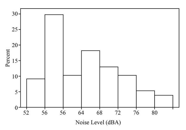
With a positive skew, the histogram is bimodal but near to unimodal. Almost one-third of the data values are concentrated in the class interval 50-60.
Compute five-number summary
The five-number summary is smallest \({x_i}\), lower fourth, median, upper fourth and largest\({x_i}\).Since sample size of test is odd, the median is the\({\left( {\frac{{n + 1}}{2}} \right)^{th}}\)ordered value when the data are in ascending order as below.
55.3 | 55.3 | 55.3 | 55.9 | 55.9 | 55.9 | 55.9 | 56.1 | 56.1 | 56.1 | 56.1 |
56.1 | 56.1 | 56.8 | 56.8 | 57.0 | 57.0 | 57.0 | 57.8 | 57.8 | 57.8 | 57.9 |
57.9 | 57.9 | 58.8 | 58.8 | 58.8 | 59.8 | 59.8 | 59.8 | 62.2 | 62.2 | 63.8 |
63.8 | 63.8 | 63.9 | 63.9 | 63.9 | 64.7 | 64.7 | 64.7 | 65.1 | 65.1 | 65.1 |
65.3 | 65.3 | 65.3 | 65.3 | 67.4 | 67.4 | 67.4 | 67.4 | 68.7 | 68.7 | 68.7 |
68.7 | 69.0 | 70.4 | 70.4 | 71.2 | 71.2 | 71.2 | 73.0 | 73.0 | 73.1 | 73.1 |
74.6 | 74.6 | 74.6 | 74.6 | 79.3 | 79.3 | 79.3 | 79.3 | 83.0 | 83.0 | 83.0 |
The smallest value is: 55.3 and the largest value is: 83.
Let \(\tilde x\) be the required median. Use the formula to calculate median when n is odd,
\(\tilde x = {\left( {\frac{{n + 1}}{2}} \right)^{th}}\,ordered\,value\)
\(\begin{aligned}\tilde x &= {\left( {\frac{{77 + 1}}{2}} \right)^{th}}\\ &= {39^{th\,}}observation\\ &= 64.7\end{aligned}\)
The lower fourth is the median of smallest half of the data as the median of the data is \(\tilde x = 64.7\)so lower half contains 41 values.
55.3 | 55.3 | 55.3 | 55.9 | 55.9 | 55.9 | 55.9 | 56.1 | 56.1 | 56.1 | 56.1 |
56.1 | 56.1 | 56.8 | 56.8 | 57.0 | 57.0 | 57.0 | 57.8 | 57.8 | 57.8 | 57.9 |
57.9 | 57.9 | 58.8 | 58.8 | 58.8 | 59.8 | 59.8 | 59.8 | 62.2 | 62.2 | 63.8 |
63.8 | 63.8 | 63.9 | 63.9 | 63.9 | 64.7 | 64.7 | 64.7 | |||
Since \(n = 41\)is odd, calculate the median using the formula:
\(\tilde x = {\left( {\frac{{n + 1}}{2}} \right)^{th}}\,ordered\,value\)
\(\begin{aligned}\tilde x &= {\left( {\frac{{41 + 1}}{2}} \right)^{th}}\,ordered\,value\\ &= {21^{th\,}}observation\\ &= 57.8\end{aligned}\)
Similarly, the upper fourth is the median of largest half of the data as the median of the data is\(\tilde x = 64.7\) so it contains 36 values.
65.1 | 65.1 | 65.1 | 65.3 | 65.3 | 65.3 | 65.3 | 67.4 | 67.4 | 67.4 | 67.4 |
68.7 | 68.7 | 68.7 | 68.7 | 69.0 | 70.4 | 70.4 | 71.2 | 71.2 | 71.2 | 73.0 |
73.0 | 73.1 | 73.1 | 74.6 | 74.6 | 74.6 | 74.6 | 79.3 | 79.3 | 79.3 | 79.3 |
83.0 | 83.0 | 83.0 | ||||||||
Since \(n = 36\)is even, calculate the median using the formula:
\(\tilde x = \frac{{{{\left( {\frac{n}{2}} \right)}^{th}} + {{\left( {\frac{n}{2} + 1} \right)}^{th}}\,ordered\,value}}{2}\)
\(\begin{aligned}\tilde x &= \frac{{{{\left( {\frac{{36}}{2}} \right)}^{th}} + {{\left( {\frac{{36}}{2} + 1} \right)}^{th}}ordered\,value}}{2}\\ &= \frac{{\left( {70.4 + 71.2} \right)}}{2}\\ &= 70.8\end{aligned}\)
Thus, the five-number summary to construct boxplot are as follows:
Smallest \({x_i}\): 55.3, lower fourth: 57.8, median: 64.7, upper fourth: 70.8,
largest \({x_i}\): 83.
Construct box plot of measurements for the given data and draw conclusion
Following are the steps to make boxplot by hand:
1. Draw a plot line of range 55 to 85.
2. Draw three horizontal lines that consists of first quartile, second quartile and third quartile and make two vertical lines to make it in rectangular form like a box for given data.
3. Draw whiskers on both sides of a boxplot and set the minimum and maximum value with respect to the obtained lower fence and upper fence.

Over 30 million students worldwide already upgrade their learning with 魅影直播!