/*! This file is auto-generated */ .wp-block-button__link{color:#fff;background-color:#32373c;border-radius:9999px;box-shadow:none;text-decoration:none;padding:calc(.667em + 2px) calc(1.333em + 2px);font-size:1.125em}.wp-block-file__button{background:#32373c;color:#fff;text-decoration:none} Q35E Mercury is a persistent and disp... [FREE SOLUTION] | 魅影直播

魅影直播

Mercury is a persistent and dispersive environmental contaminantfound in many ecosystems around the world.When released as an industrial by-product, it often finds itsway into aquatic systems where it can have deleteriouseffects on various avian and aquatic species. The accompanyingdata on blood mercury concentration (mg/g) for adult

females near contaminated rivers in Virginia was read from a graph in the article 鈥淢ercury Exposure Effects the Reproductive Success of a Free-Living Terrestrial Songbird, the Carolina Wren鈥 (The Auk, 2011: 759鈥769;this is a publication of the American Ornithologists鈥 Union).

.20 .22 .25 .30 .34 .41 .55 .56

1.42 1.70 1.83 2.20 2.25 3.07 3.25

a. Determine the values of the sample mean and sample median and explain why they are different. (Hint:\(\sum {{{\bf{x}}_{\bf{1}}}{\bf{ = 18}}{\bf{.55}}} \))

b. Determine the value of the 10% trimmed mean and compare to the mean and median.

c. By how much could the observation .20 be increased without impacting the value of the sample median?

Short Answer

Expert verified
  1. The sample mean for x is 1.237 mg/g.The median value of x is 0.56 mg/g. The two values are different due to positive skewness in the distribution of values.
  2. The 10% trimmed mean is 1.118mg/g. The value lies between median and mean value of 0.56 and 1.237 respectively.
  3. The observation .20 can be increased to 0.36 without impacting the value of the sample median.

Step by step solution

01

Given information

The data on the blood mercury concentration (mg/g) for adult females near contaminated rivers in Virginia is provided.

02

Compute the sample mean and sample median

  1. Let x represents the blood mercury concentration (mg/g) for adult females near contaminated rivers in Virginia.

The sample mean is computed as,

\(\begin{array}{c}\bar x &=& \frac{{\sum {{x_i}} }}{n}\\ &=& \frac{{0.20 + 0.22 + 0.25 + ... + 3.25}}{{15}}\\ &=& \frac{{18.55}}{{15}}\\ &=& 1.237\end{array}\)

Thus, the sample mean for x is 1.237 mg/g.

For the odd number of observations, the median value is computed as,

\(\begin{array}{c}\tilde x &=& {\left( {\frac{{n + 1}}{2}} \right)^{th}}{\rm{ordered}}\;{\rm{value}}\\ &=& {\left( {\frac{{15 + 1}}{2}} \right)^{th}}{\rm{ordered}}\;{\rm{value}}\\ &=& {\left( 8 \right)^{th}}{\rm{ordered}}\;{\rm{value}}\end{array}\)

Thus, the median value of x is 0.56.

The sample mean represents the average of values

The sample median separates the data into equal halves.

The two values are different in magnitude because the distribution of values is not symmetric but positively skewed.

03

Compute the 10% trimmed mean

b.

10% trimmed mean is the mean value obtained after removing 10% of the extreme (largest and smallest value each) from the data.

In this case, 10% of 15 is 1.5. Thus, the following procedure is carried out to compute trimmed mean.

A 10% trimmed mean is computed by removing the smallest and the largest observation from the data.

Remove one extreme value from each end to obtain the data as follows,

0.22

0.25

0.3

0.34

0.41

0.55

0.56

1.42

1.7

1.83

2.2

2.25

3.07

The sample mean is computed as,

\(\begin{array}{c}{{\bar x}_{\left( {tr1} \right)}} &=& \frac{{\sum {{x_i}} }}{n}\\ &=& \frac{{0.22 + 0.25 + ... + 3.07}}{{13}}\\ &=& 1.162\end{array}\)

Now, again remove the smallest and largest value from the remaining dataset.

The data after removing is as follows,

0.25

0.3

0.34

0.41

0.55

0.56

1.42

1.7

1.83

2.2

2.25

The sample mean is computed as,

\(\begin{array}{c}{{\bar x}_{\left( {tr2} \right)}} &=& \frac{{\sum {{x_i}} }}{n}\\ &=& \frac{{0.25 + 0.3 + ... + 2.25}}{{11}}\\ &=& 1.0736\end{array}\)

Now, the 10% trimmed mean for the data is computed as,

\(\begin{array}{c}{{\bar x}_{tr}} &=& \frac{{{{\bar x}_{\left( {tr1} \right)}} + {{\bar x}_{\left( {tr2} \right)}}}}{2}\\ &=& \frac{{1.162 + 1.0736}}{2}\\ &=& 1.118\end{array}\)

Thus, the 10% trimmed mean is 1.118.

Therefore, it can be observed that the trimmed mean (1.118) falls between the median value (0.56) and the mean value (1.237).

04

Obtain the maximum value to which 0.20 can be increased to keep sample median constant

The median value of x is 0.56.

The value that the observation .20 be increased without impacting the value of the sample median is computed as,

\(\begin{array}{c}\frac{{0.20}}{{0.56}} = 0.357\\ \approx 0.36\end{array}\)

Thus, the observation .20 can be increased to 0.36 without impacting the value of the sample median.

Unlock Step-by-Step Solutions & Ace Your Exams!

  • Full Textbook Solutions

    Get detailed explanations and key concepts

  • Unlimited Al creation

    Al flashcards, explanations, exams and more...

  • Ads-free access

    To over 500 millions flashcards

  • Money-back guarantee

    We refund you if you fail your exam.

Over 30 million students worldwide already upgrade their learning with 魅影直播!

One App. One Place for Learning.

All the tools & learning materials you need for study success - in one app.

Get started for free

Most popular questions from this chapter

a. If a constant cis added to each \({x_i}\)in a sample, yielding \({y_i} = {x_i} + c\), how do the sample mean and median of the \({y_i}'s\)relate to the mean and median of the\({x_i}'s\)? Verify your conjectures.

b. If each \({x_i}\)is multiplied by a constant c,yielding \({y_i} = c{x_i}\), answer the question of part (a). Again, verify your conjectures.

Exposure to microbial products, especially endotoxin, may have an impact on vulnerability to allergic diseases. The article 鈥淒ust Sampling Methods for Endotoxin鈥擜n Essential, But Underestimated Issue鈥 (Indoor Air,2006: 20鈥27) considered various issues associated with determining endotoxin concentration. The following data on concentration (EU/mg) in settled dust for one sample of urban homes and another of farm homes was kindly supplied by the authors of the cited article.

U: 6.0 5.0 11.0 33.0 4.0 5.0 80.0 18.0 35.0 17.0 23.0

F: 4.0 14.0 11.0 9.0 9.0 8.0 4.0 20.0 5.0 8.9 21.0

9.2 3.0 2.0 0.3

  1. Determine the sample mean for each sample. How do they compare?
  2. Determine the sample median for each sample. How do they compare? Why is the median for the urban sample so different from the mean for that sample?
  3. Calculate the trimmed mean for each sample by deleting the smallest and largest observation. What are the corresponding trimming percentages? How do the values of these trimmed means compare to the corresponding means and medians?

Give one possible sample of size 4 from each of the following

populations:

a. All daily newspapers published in the United States

b. All companies listed on the New York Stock Exchange

c. All students at your college or university

d. All grade point averages of students at your college or university

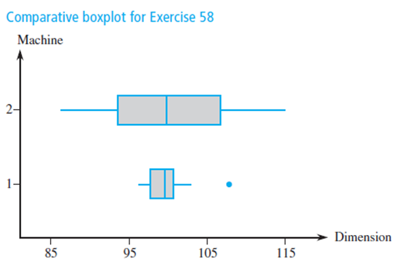
A company utilizes two different machines to manufacture parts of a certain type. During a single shift, a sample of n=20 parts produced by each machine is obtained, and the value of a particular critical dimension for each part is determined. The comparative boxplot at the bottom of this page is constructed from the resulting data. Compare and contrast the two samples.

The accompanying data set consists of observations,on shower-flow rate (L/min) for a sample of n=129,houses in Perth, Australia (鈥淎n Application of Bayes,Methodology to the Analysis of Diary Records in a

Water Use Study,鈥 J. Amer. Stat. Assoc., 1987: 705鈥711):

4.6 12.3 7.1 7.0 4.0 9.2 6.7 6.9 11.5 5.1

11.2 10.5 14.3 8.0 8.8 6.4 5.1 5.6 9.6 7.5

7.5 6.2 5.8 2.3 3.4 10.4 9.8 6.6 3.7 6.4

8.3 6.5 7.6 9.3 9.2 7.3 5.0 6.3 13.8 6.2

5.4 4.8 7.5 6.0 6.9 10.8 7.5 6.6 5.0 3.3

7.6 3.9 11.9 2.2 15.0 7.2 6.1 15.3 18.9 7.2

5.4 5.5 4.3 9.0 12.7 11.3 7.4 5.0 3.5 8.2

8.4 7.3 10.3 11.9 6.0 5.6 9.5 9.3 10.4 9.7

5.1 6.7 10.2 6.2 8.4 7.0 4.8 5.6 10.5 14.6

10.8 15.5 7.5 6.4 3.4 5.5 6.6 5.9 15.0 9.6

7.8 7.0 6.9 4.1 3.6 11.9 3.7 5.7 6.8 11.3

9.3 9.6 10.4 9.3 6.9 9.8 9.1 10.6 4.5 6.2

8.3 3.2 4.9 5.0 6.0 8.2 6.3 3.8 6.0

  1. Construct a stem-and-leaf display of the data.
  2. What is a typical, or representative, flow rate?
  3. Does the display appear to be highly concentrated or spread out?
  4. Does the distribution of values appear to be reasonably symmetric? If not, how would you describe the departure from symmetry?
  5. Would you describe any observation as being far from the rest of the data (an outlier)?
See all solutions

Recommended explanations on Math Textbooks

View all explanations

What do you think about this solution?

We value your feedback to improve our textbook solutions.

Study anywhere. Anytime. Across all devices.