/*! This file is auto-generated */ .wp-block-button__link{color:#fff;background-color:#32373c;border-radius:9999px;box-shadow:none;text-decoration:none;padding:calc(.667em + 2px) calc(1.333em + 2px);font-size:1.125em}.wp-block-file__button{background:#32373c;color:#fff;text-decoration:none} Q8 E Tensile-strength tests were carr... [FREE SOLUTION] | 魅影直播

魅影直播

Tensile-strength tests were carried out on two different grades of wire rod (鈥淔luidized Bed Patenting of Wire Rods,鈥 Wire J., June \(1977: 56 - 61)\), resulting in the accompanying data

Sample

Sample Mean Sample

Grade Size (kg/mm2 ) SD

\(\overline {\underline {\begin{array}{*{20}{l}}{ AISI 1064}&{m = 129}&{\bar x = 107.6}&{{s_1} = 1.3}\\{ AISI 1078}&{n = 129}&{\bar y = 123.6}&{{s_2} = 2.0}\\{}&{}&{}&{}\end{array}} } \)

a. Does the data provide compelling evidence for concluding that true average strength for the \(1078\) grade exceeds that for the \(1064\) grade by more than \(10kg/m{m^2}\) ? Test the appropriate hypotheses using a significance level of \(.01\).

b. Estimate the difference between true average strengths for the two grades in a way that provides information about precision and reliability

Short Answer

Expert verified

the solution is

a)There is adequate evidence to support the allegation that the genuine average strength of the \(1078\)grade is more than \(10kg/m{m^2}\) more than that of the \(1064\) grade.

b)\(( - 16.4116, - 15.5884)\)

Step by step solution

01

test the appropriate hypotheses

  1. given:

\(\begin{array}{l}{{\bar x}_1} = 107.6\\{{\bar x}_2} = 123.6\\{s_1} = 1.3\\{s_2} = 2.0\end{array}\)

\(\begin{array}{l}{n_1} = 129\\{n_2} = 129\\\alpha = 0.01\end{array}\)

We may use the \(z\)-test because the samples are large \(\left( {n > 30} \right)\). (instead of a t-test).

Assumption: exceed by more than \(10\)

Either the null hypothesis or the alternative hypothesis is asserted. The null hypothesis and the alternative hypothesis are diametrically opposed. An equality must be included in the null hypothesis.

\(\begin{array}{l}{H_0}:{\mu _1} - {\mu _2} = - 10\\{H_a}:{\mu _1} - {\mu _2} > - 10\end{array}\)

Determine the value of the test statistic:

\(z = \frac{{{{\bar x}_1} - {{\bar x}_2} - \left( {{\mu _1} - {\mu _2}} \right)}}{{\sqrt {\frac{{s_1^2}}{{{n_1}}} + \frac{{s_2^2}}{{{n_2}}}} }} = \frac{{107.6 - 123.6 - ( - 10)}}{{\sqrt {\frac{{1.{3^2}}}{{129}} + \frac{{2.{0^2}}}{{129}}} }} \approx - 28.57\)

If the null hypothesis is true, the \(P\)-value is the probability of getting a result more extreme or equal to the standardized test statistic \(z\). Using the normal probability table, determine the probability.

\(P = P(Z < - 28.57 or Z > 28.57) = 2P(Z < - 28.57) \approx 2(0) = 0\)

The null hypothesis is rejected if the P-value is less than the alpha significance level.

\(P < 0.01 \Rightarrow Reject {H_0}\)

There is adequate evidence to support the allegation that the genuine average strength of the \(1078\)grade is more than \(10kg/m{m^2}\) more than that of the \(1064\) grade.

02

given

b)

\(\begin{array}{l}{{\bar x}_1} = 107.6\\{{\bar x}_2} = 123.6\\{s_1} = 1.3\\{s_2} = 2.0\end{array}\)

\(\begin{array}{l}{n_1} = 129\\{n_2} = 129\end{array}\)

We will compute a \(95\% \) confidence interval, confidence intervals with other confidence levels can be calculated similarly.

\(c = 95\% = 0.95\)

03

confidence interval

for confidence interval\(1 - \alpha = 0.95,\) determine \({z_{\alpha /2}} = {z_{0.025}}\) using the normal probability table ( look up \(0.025\) in the table, the \(z\)-score is then the found \(z\)-score with opposite sign):

\({z_{\alpha /2}} = 1.96\)

The margin of error then becomes:

\({z_{\alpha /2}} = 1.96E = {z_{\alpha /2}} \times \sqrt {\frac{{\sigma _1^2}}{{{n_1}}} + \frac{{\sigma _2^2}}{{{n_2}}}} = 1.96 \times \sqrt {\frac{{1.{3^2}}}{{129}} + \frac{{2.{0^2}}}{{129}}} \)\( \approx 0.4116\)

The endpoints of the confidence interval of \({\mu _1} - {\mu _2}\) are:

\(\begin{array}{l}\left( {{{\bar x}_1} - {{\bar x}_2}} \right) - E = (107.6 - 123.6) - 0.4116 = - 16 - 0.4116 = - 16.4116\\\left( {{{\bar x}_1} - {{\bar x}_2}} \right) + E = (107.6 - 123.6) + 0.4116 = - 16 + 0.4116 = - 15.5884\end{array}\)

04

conclusion

a)There is adequate evidence to support the allegation that the genuine average strength of the \(1078\)grade is more than \(10kg/m{m^2}\) more than that of the \(1064\) grade.

b)\(( - 16.4116, - 15.5884)\)

Unlock Step-by-Step Solutions & Ace Your Exams!

  • Full Textbook Solutions

    Get detailed explanations and key concepts

  • Unlimited Al creation

    Al flashcards, explanations, exams and more...

  • Ads-free access

    To over 500 millions flashcards

  • Money-back guarantee

    We refund you if you fail your exam.

Over 30 million students worldwide already upgrade their learning with 魅影直播!

One App. One Place for Learning.

All the tools & learning materials you need for study success - in one app.

Get started for free

Most popular questions from this chapter

Anorexia Nervosa (AN) is a psychiatric condition leading to substantial weight loss among women who are fearful of becoming fat. The article "Adipose Tissue Distribution After Weight Restoration and Weight Maintenance in Women with Anorexia Nervosa" (Amer. J. of ClinicalNutr., 2009: 1132-1137) used whole-body magnetic resonance imagery to determine various tissue characteristics for both an AN sample of individuals who had undergone acute weight restoration and maintained their weight for a year and a comparable (at the outset of the study) control sample. Here is summary data on intermuscular adipose tissue (IAT; kg).

Assume that both samples were selected from normal distributions.

a. Calculate an estimate for true average IAT under the described AN protocol, and do so in a way that conveys information about the reliability and precision of the estimation.

b. Calculate an estimate for the difference between true average AN IAT and true average control IAT, and do so in a way that conveys information about the reliability and precision of the estimation. What does your estimate suggest about true average AN IAT relative to true average control IAT?

The degenerative disease osteoarthritis most frequently affects weight-bearing joints such as the knee. The article "Evidence of Mechanical Load Redistribution at the Knee Joint in the Elderly When Ascending Stairs and Ramps" (Annals of Biomed. Engr., \(2008: 467 - 476\)) presented the following summary data on stance duration (ms) for samples of both older and younger adults.

\(\begin{array}{*{20}{l}}{Age\;\;\;\;\;\;\;Sample Size\;\;Sample Mean\;\;Sample SD}\\{\;Older\;\;\;\;\;28\;\;\;\;\;\;\;\;\;\;\;\;\;\;\;\;\;\;\;\;801\;\;\;\;\;\;\;\;\;\;\;\;\;\;\;\;\;117}\\{Younger\;16\;\;\;\;\;\;\;\;\;\;\;\;\;\;\;\;\;\;\;\;780\;\;\;\;\;\;\;\;\;\;\;\;\;\;\;\;\;72}\end{array}\)

Assume that both stance duration distributions are normal.

a. Calculate and interpret a\(99\% \)CI for true average stance duration among elderly individuals.

b. Carry out a test of hypotheses at significance level\(.05\)to decide whether true average stance duration is larger among elderly individuals than among younger individuals.

Many freeways have service (or logo) signs that give information on attractions, camping, lodging, food, and gas services prior to off-ramps. These signs typically do not provide information on distances. The article "Evaluation of Adding Distance Information to Freeway-Specific Service (Logo) Signs" \((J\). of Transp. Engr., 2011: 782-788) reported that in one investigation, six sites along Virginia interstate highways where service signs are posted were selected. For each site, crash data was obtained for a three-year period before distance information was added to the service signs and for a one-year period afterward. The number of crashes per year before and after the sign changes were as follows:

\(\begin{array}{*{20}{l}}{Before:\;\;15\;26\;66\;115\;62\;64}\\{After:\;\;\;\;\;16\;24\;42\;80\;\;78\;73}\end{array}\)

a. The cited article included the statement "A paired\(t\)test was performed to determine whether there was any change in the mean number of crashes before and after the addition of distance information on the signs." Carry out such a test. (Note: The relevant normal probability plot shows a substantial linear pattern.)

b. If a seventh site were to be randomly selected among locations bearing service signs, between what values would you predict the difference in number of crashes to lie?

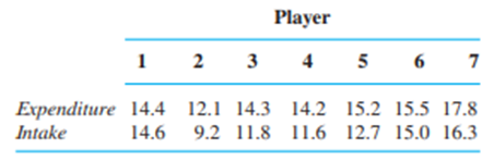
How does energy intake compare to energy expenditure? One aspect of this issue was considered in the article 鈥淢easurement of Total Energy Expenditure by the Doubly Labelled Water Method in Professional Soccer Players鈥 (J. of Sports Sciences, 2002: 391鈥397), which contained the accompanying data (MJ/day).

Test to see whether there is a significant difference between intake and expenditure. Does the conclusion depend on whether a significance level of .05, .01, or .001 is used?

Pilates is a popular set of exercises for the treatment of individuals with lower back pain. The method has six basic principles: centering, concentration, control, precision, flow, and breathing. The article 鈥淓fficacy of the Addition of Modified Pilates Exercises to a Minimal Intervention in Patients with Chronic Low Back Pain: A Randomized Controlled Trial鈥 (Physical Therapy, \(2013:309 - 321\)) reported on an experiment involving \(86\) subjects with nonspecific low back pain. The participants were randomly divided into two groups of equal size. The first group received just educational materials, whereas the second group participated in \(6\) weeks of Pilates exercises. The sample mean level of pain (on a scale from \(0\) to \(10\)) for the control group at a \(6\)-week follow-up was \(5.2\) and the sample mean for the treatment group was \(3.1\); both sample standard deviations were \(2.3\).

a. Does it appear that true average pain level for the control condition exceeds that for the treatment condition? Carry out a test of hypotheses using a significance level of \(.01\) (the cited article reported statistical significance at this a, and a sample mean difference of \(2.1\) also suggests practical significance)

b. Does it appear that true average pain level for the control condition exceeds that for the treatment condition by more than \(1\)? Carry out a test of appropriate hypotheses

See all solutions

Recommended explanations on Math Textbooks

View all explanations

What do you think about this solution?

We value your feedback to improve our textbook solutions.

Study anywhere. Anytime. Across all devices.