/*! This file is auto-generated */ .wp-block-button__link{color:#fff;background-color:#32373c;border-radius:9999px;box-shadow:none;text-decoration:none;padding:calc(.667em + 2px) calc(1.333em + 2px);font-size:1.125em}.wp-block-file__button{background:#32373c;color:#fff;text-decoration:none} Q36SE Cortisol is a hormone that plays... [FREE SOLUTION] | 魅影直播

魅影直播

Cortisol is a hormone that plays an important role in mediating stress. There is growing awareness that exposure of outdoor workers to pollutants may impact cortisol levels. The article 鈥淧lasma Cortisol Concentration and Lifestyle in a Population of Outdoor Workers鈥 (Intl. J. of Envir. Health Res., 2011: 62鈥71) reported on a study involving three groups of police officers: (1) traffic police (TP), (2) drivers (D), and (3) other duties (O). Here is summary data on cortisol concentration (ng/ml) for a subset of the officers who neither drank nor smoked.

Group

Sample Size

Mean

SD

TP

47

174.7

50.9

D

36

160.2

3702

O

50

153.5

45.9

Assuming that the standard assumptions for one-way ANOVA are satisfied, carry out a test at significance level .05 to decide whether true average cortisol concentration is different for the three groups. (Note: The investigators used more sophisticated statistical methodology (multiple regression) to assess the impact of age, length of employment, and drinking and smoking status on cortisol concentration; taking these factors into account, concentration appeared to be significantly higher in the TP group than in the other two groups.)

Short Answer

Expert verified

There is not sufficient evidence to support the claim that the true average cortisol concentration is different for the three groups.

Step by step solution

01

Finding value of ANOVA F

\(\begin{aligned}{l}{n_1} = 47\\{n_2} = 36\\{n_3} = 50\\\overline {{x_1}} = 174.7\\\overline {{x_2}} = 160.2\\\overline {{x_3}} = 153.5\\{s_1} = 50.9\\{s_2} = 37.2\\{s_3} = 45.9\\\alpha = 0.05\end{aligned}\)

The overall mean is the sum of all values divided by the number of values:

\(\overline x = \frac{{{n_1}\overline {{x_1}} + {n_2}\overline {{x_2}} + {n_3}\overline {{x_3}} }}{N} = \frac{{47(174.7) + 36(160.2) + 50(153.5)}}{{47 + 3 + 50}} \approx 162.8053\)

The mean square for treatment is:

\(\begin{aligned}{l}MSTr = \frac{{{n_1}{{(\overline {{x_1}} - \overline x )}^2} + {n_2}{{(\overline {{x_2}} - \overline x )}^2} + {n_2}{{(\overline {{x_3}} - \overline x )}^2}}}{{I - 1}}\\ = \frac{{47{{(147.7 - 162.8053)}^2} + 36{{(160.2 - 162.8053)}^2} + 50{{(153.5 - 162.8053)}^2}}}{{3 - 1}} = 5611.7632\end{aligned}\)

The mean square error is:

\(\begin{aligned}{l}MSE = \frac{{({n_1} - 1)s_1^2 + ({n_2} - 1)s_2^2 + ({n_3} - 1)s_3^2}}{{N - I}}\\ = \frac{{(47 - 1){{(50.9)}^2} + (36 - 1){{(37.2)}^2} + (50 - 1){{(45.9)}^2}}}{{(47 + 36 + 50) - 3}} = 2083.4258\end{aligned}\)

The ANOVA F statistic is the ratio of the MSTr and MSE:

\(F = \frac{{MSTr}}{{MSE}} = \frac{{5611.7632}}{{2083.4258}} \approx 2.694\)

02

Checking whether true average cortisol concentration is different for the three groups using P-Value

The P-value is the probability of obtaining the value of the test statistic, or a value more extreme. The P-value is the number (or interval) in the column title of the F-distribution table in the appendix containing the F-value in the row\(dfn = I - 1 = 3 - 1 = 2\)and \(dfd = N - I = 47 + 36 + 50 - 3 = 130 > 100:\)

\(0.050 < P < 0.100\)

If the P-value is less than the significance level, then reject the null hypothesis.

\(P > 0.05 \Rightarrow \)Fail to reject\({H_0}\)

There is not sufficient evidence to support the claim that the true average cortisol concentration is different for the three groups.

Unlock Step-by-Step Solutions & Ace Your Exams!

  • Full Textbook Solutions

    Get detailed explanations and key concepts

  • Unlimited Al creation

    Al flashcards, explanations, exams and more...

  • Ads-free access

    To over 500 millions flashcards

  • Money-back guarantee

    We refund you if you fail your exam.

Over 30 million students worldwide already upgrade their learning with 魅影直播!

One App. One Place for Learning.

All the tools & learning materials you need for study success - in one app.

Get started for free

Most popular questions from this chapter

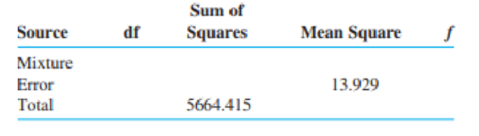
An experiment was carried out to compare electrical resitivity for six different low-permeability concrete bridge deck mixtures. There were \(26\)measurements on concrete cylinders for each mixture; these were obtained days \(28\)after casting.The entries in the accompanying ANOVA table are based on information in the article 鈥淚n-place Resitivity of Bridge Deck Concrete Mixtures鈥(ACI Matrerials j.,2009: 114-122).Fill in the remaining entries and test appropriate hypothese.

The critical flicker frequency \(\left( {cff} \right)\) is the highest frequency at which a person can detect the flicker in a flickering light source. At frequencies above the cff, the light source appear to be continuous even though it is actually flickering. An investigation carried out to see whether true average cff depends on iris color yielded the following data (based on the article 鈥淭he Effects of Iris Color on Critical Flicker Frequency鈥.

Iris color

1.Brown

2.Green

3.Blue

\({\bf{26}}.{\bf{8}}\)

\({\bf{26}}.{\bf{4}}\)

\({\bf{25}}.{\bf{7}}\)

\({\bf{27}}.{\bf{9}}\)

\({\bf{24}}.{\bf{2}}\)

\({\bf{27}}.{\bf{2}}\)

\({\bf{23}}.{\bf{7}}\)

\({\bf{28}}.{\bf{0}}\)

\({\bf{29}}.{\bf{9}}\)

\({\bf{25}}.{\bf{0}}\)

\({\bf{26}}.{\bf{9}}\)

\({\bf{28}}.{\bf{5}}\)

\({\bf{26}}.{\bf{3}}\)

\({\bf{29}}.{\bf{1}}\)

\({\bf{29}}.{\bf{4}}\)

\({\bf{24}}.{\bf{8}}\)

\({\bf{28}}.{\bf{3}}\)

\({\bf{25}}.{\bf{7}}\)

\({\bf{24}}.{\bf{5}}\)

\({J_i}\)

\({\bf{8}}\)

\({\bf{5}}\)

\({\bf{6}}\)

\({x_i}\)

\({\bf{204}}.{\bf{7}}\)

\({\bf{134}}.{\bf{6}}\)

\({\bf{169}}.{\bf{0}}\)

\({\overline x _i}\)

\({\bf{25}}.{\bf{59}}\)

\({\bf{26}}.{\bf{92}}\)

\({\bf{28}}.{\bf{17}}\)

\(n = 19,{x_{..}} = 508.3\)

  1. State and test the relevant hypotheses at significance level\(.05\)(Hint:\(\sum {\sum {{x_{ij}}^2} = 13659.67,CF = 13598.36} \))
  2. Investigate difference between iris colors with respect to mean cff.

In an experiment to compare the tensile strengths of different type of\({\bf{I = 5}}\) copper wire, \({\bf{J = 4}}\) samples of each type were used. The between-samples and within- sample estimates of \({{\bf{\sigma }}^{\bf{2}}}\) were computed as \({\bf{MS}}{{\bf{T}}_{\bf{r}}}{\bf{ = 2673}}{\bf{.3}}\) and respectively. Use the F test at level. to test \({{\bf{H}}_{\bf{0}}}\,{\bf{:}}\,\,{{\bf{\mu }}_{\bf{1}}}{\bf{ = }}{{\bf{\mu }}_{\bf{2}}}{\bf{ = }}{{\bf{\mu }}_{\bf{3}}}{\bf{ = }}{{\bf{\mu }}_{\bf{4}}}{\bf{ = }}{{\bf{\mu }}_{\bf{5}}}\)versus \({{\bf{H}}_{\bf{a}}}{\bf{:}}\)at least two \({{\bf{\mu }}_{\bf{i}}}{\bf{'s}}\) are unequal.

Suppose the compression strength observation on the fourth type of box in Example \(10.1\)had been \(655.1,\,748.7,\,662.4,\,679.0,\,706.9,\,and\,640.0\) and (obtained by adding \(120\) to each previous \({x_{4j}}\)). Assuming no change in the remaining observations, carry out an F test with \(\alpha = 0.5.\)

Six samples of each of four types of cereal grain grown in a certain region were analyzed to determine thiamin content, resulting in the following data \((\mu g/g):\)

Wheat \(5.2\) \(4.5\) \(6.0\) \(6.1\) \(6.7\) \(5.8\)

Barley \(6.5\) \(8.0\) \(6.1\) \(7.5\) \(5.9\) \(5.6\)

Maize \(5.8\) \(4.7\) \(6.4\) \(4.9\) \(6.0\) \(5.2\)

Oats \(8.3\) \(6.1\) \(7.8\) \(7.0\) \(5.5\) \(7.2\)

Does this data suggest that at least two of the grains differ with respect to true average thiamin content? Use a level \(\alpha = .05\)

See all solutions

Recommended explanations on Math Textbooks

View all explanations

What do you think about this solution?

We value your feedback to improve our textbook solutions.

Study anywhere. Anytime. Across all devices.