/*! This file is auto-generated */ .wp-block-button__link{color:#fff;background-color:#32373c;border-radius:9999px;box-shadow:none;text-decoration:none;padding:calc(.667em + 2px) calc(1.333em + 2px);font-size:1.125em}.wp-block-file__button{background:#32373c;color:#fff;text-decoration:none} Q74E Once an individual has been infe... [FREE SOLUTION] | 魅影直播

魅影直播

Once an individual has been infected with a certain disease, let \({\rm{X}}\) represent the time (days) that elapses before the individual becomes infectious. The article proposes a Weibull distribution with \({\rm{\alpha = 2}}{\rm{.2}}\), \({\rm{\beta = 1}}{\rm{.1}}\), and \({\rm{\gamma = 0}}{\rm{.5}}\).

a. Calculate \({\rm{P(1 < X < 2)}}\).

b. Calculate \({\rm{P(X > 1}}{\rm{.5)}}\).

c. What is the \({\rm{90th}}\) percentile of the distribution?

d. What are the mean and standard deviation of \({\rm{X}}\)?

Short Answer

Expert verified

a.The probability then becomes:

\(\begin{array}{c}{\rm{P(1 < X < 2) = 0}}{\rm{.699948}}\\{\rm{ = 69}}{\rm{.9948\% }}\end{array}\)

b.The probability then becomes:

\(\begin{array}{c}{\rm{P(X > 1}}{\rm{.5) = 0}}{\rm{.444484}}\\{\rm{ = 44}}{\rm{.4484\% }}\end{array}\)

c. The \({\rm{90th}}\) percentile of the distribution is \(2.107\)

d. The mean and standard deviation

\(\begin{array}{l}{\rm{\mu = 1}}{\rm{.474187}}\\{\rm{\sigma = 0}}{\rm{.467443}}\end{array}\)

Step by step solution

01

Definition of Weibull distribution

The Weibull Distribution is a continuous probability distribution that can be used to analyze life statistics, model failure times, and determine product reliability.

02

Calculate the equation

Given: \({\rm{X}}\)has a general Weibull distribution with

\(\begin{array}{l}{\rm{\alpha = 2}}{\rm{.2}}\\{\rm{\beta = 1}}{\rm{.1}}\\{\rm{\gamma = 0}}{\rm{.5P(1 < X < 2)}}\end{array}\)

Then we know that \({\rm{Y = X - }}\gamma \) has a (regular) Weibull distribution with \({\rm{\alpha = 2}}{\rm{.2}}\) and \({\rm{\beta = 1}}{\rm{.1}}\), thus:

\({\rm{X = Y + }}\gamma \)

Rewrite the given probability in terms of \({\rm{Y}}\):

\(\begin{aligned} P(1 < X < 2) &= P(1 < Y + \gamma < {\rm{2)}}\\ &= P(1 - \gamma < {\rm{Y}} < 2 - \gamma )\\ &= P(Y < 2 - \gamma ){\rm{ - P(Y}} \le 1 - \gamma )\\ &= P(Y \le 2 - \gamma ){\rm{ - P(Y}} \le 1 - \gamma )\\ &= P(Y \le 2 - 0.5){\rm{ - P(Y}} \le 1 - 0.5)\\ &= P(Y \le 1.5){\rm{ - P(Y}} \le 0.5)\\ &= {\rm{F(1}}{\rm{.5) - F(0}}{\rm{.5)}}\end{aligned}\)

Cumulative distribution function of a (regular) Weibull distribution:

\({\rm{F(x;\alpha ,\beta ) = }}\left\{ {\begin{array}{*{20}{c}}0&{x < 0}\\{1 - {{\rm{e}}^{{\rm{ - (x/\beta }}{{\rm{)}}^{\rm{\alpha }}}}}}&{x \ge 0}\end{array}} \right.\)

Evaluate at \({\rm{x = 1}}{\rm{.5}}\) and \({\rm{x = 0}}{\rm{.5}}\):

\(\begin{array}{c}{\rm{F(1}}{\rm{.5;\alpha ,\beta ) = F(1}}{\rm{.5;2}}{\rm{.2,1}}{\rm{.1)}}\\{\rm{ = 1 - }}{{\rm{e}}^{{\rm{ - (1}}{\rm{.5/1}}{\rm{.1}}{{\rm{)}}^{{\rm{2}}{\rm{.2}}}}}} \approx 0.861724\\F(0.5;\alpha ,\beta ) = {\rm{F(0}}{\rm{.5;2}}{\rm{.2,1}}{\rm{.1)}}\\{\rm{ = 1 - }}{{\rm{e}}^{{\rm{ - (0}}{\rm{.5/1}}{\rm{.1}}{{\rm{)}}^{{\rm{2}}{\rm{.2}}}}}} \approx 0.161776\end{array}\)

Therefore,The probability then becomes:

\(\begin{aligned}P(1 < X < 2) &= F(1}}{\rm{.5) - F(0}}{\rm{.5)}}\\ &= 0 {\rm{.861724 - 0}}{\rm{.161776}}\\ &= 0{\rm{.699948}}\\ &= 69{\rm{.9948\% }}\end{aligned}\)

03

Calculate the equation

Given: The Weibull distribution for \({\rm{X}}\) is universal.

\(\begin{array}{l}{\rm{\alpha = 2}}{\rm{.2}}\\{\rm{\beta = 1}}{\rm{.1}}\\\gamma {\rm{ = 0}}{\rm{.5P(X > 1}}{\rm{.5)}}\end{array}\)

Then we know that \({\rm{Y = X - }}\gamma \) has a (regular) Weibull distribution with \({\rm{\alpha = 2}}{\rm{.2}}\) and \({\rm{\beta = 1}}{\rm{.1}}\), thus:

\({\rm{X = Y + }}\gamma \)

Complement rule:

\({\rm{P(notA) = 1 - P(A)}}\)

Use the complement rule to rewrite the given probability in terms of \({\rm{Y}}\):

\(\begin{array}{c}{\rm{P(X}} > 1.5){\rm{ = P(Y}} + \gamma > 1.5)\\{\rm{ = P(Y > }}1.5 - \gamma )\\{\rm{ = 1 - P(Y}} \le 1.5 - \gamma )\\{\rm{ = 1 - P(Y}} \le 1.5 - 0.5)\\{\rm{ = 1 - P(Y}} \le 1)\\{\rm{ = 1 - F(1)}}\end{array}\)

A (regular) Weibull distribution's cumulative distribution function is:

\({\rm{F(x;\alpha ,\beta )}} = \left\{ {\begin{array}{*{20}{c}}0&{x < 0}\\{{\rm{1 - }}{{\rm{e}}^{{\rm{ - (x/\beta }}{{\rm{)}}^{\rm{\alpha }}}}}}&{x \ge 0}\end{array}} \right.\)

Evaluate at $x=1$ :

\(\begin{array}{c}{\rm{F(1;\alpha ,\beta ) = F(1;2}}{\rm{.2,1}}{\rm{.1)}}\\{\rm{ = 1 - }}{{\rm{e}}^{{\rm{ - (1/1}}{\rm{.1}}{{\rm{)}}^{{\rm{2}}{\rm{.2}}}}}} \approx 0.555516\end{array}\)

Therefore,The likelihood then becomes:

\(\begin{array}{c}{\rm{P(X > 1}}{\rm{.5) = 1 - F(1)}}\\{\rm{ = 1 - 0}}{\rm{.555516}}\\{\rm{ = 0}}{\rm{.444484}}\\{\rm{ = 44}}{\rm{.4484\% }}\end{array}\)

04

Explain the \({\rm{90th}}\) percentile of the distribution?

The number \({\rm{X}}\) represents the amount of time (in days) that passes before the individual becomes contagious. Also, \({\rm{X}}\) has the following Weibull distribution parameters:

\(\begin{array}{l}{\rm{\alpha = 2}}{\rm{.2}}\\{\rm{\beta = 1}}{\rm{.1}}\\\gamma = 0.5\end{array}\)

The cdf of given Weibull rv can be written as:

\({\rm{F(x) = }}\left\{ {\begin{array}{*{20}{l}}0&{x < 0}\\{{\rm{1 - }}{{\rm{e}}^{{\rm{ - ((x - 0}}{\rm{.5)/1}}{\rm{.1}}{{\rm{)}}^{{\rm{2}}{\rm{.2}}}}}}}&{x \ge 0.5}\end{array}} \right.\)

Let us denote the \({90^{{\rm{th }}}}\)percentile by \({\mathop{\rm p}\nolimits} \)

Then using the cdf, we can write \({\mathop{\rm P}\nolimits} (X \le 6)\)as:

\(\begin{array}{c}{\rm{P(X}} \le p){\rm{ = 0}}{\rm{.91 - }}{{\rm{e}}^{{\rm{ - ((p - 0}}{\rm{.5)/1}}{\rm{.1}}{{\rm{)}}^{{\rm{2}}{\rm{.2}}}}}}\\{\rm{ = 0}}{\rm{.9}}{{\rm{e}}^{{\rm{ - ((p - 0}}{\rm{.5)/1}}{\rm{.1}}{{\rm{)}}^{{\rm{2}}{\rm{.2}}}}}}\\{\rm{ = 0}}{\rm{.1}}{\left( {\frac{{{\rm{p - 0}}{\rm{.5}}}}{{{\rm{1}}{\rm{.1}}}}} \right)^{{\rm{2}}{\rm{.2}}}}\\{\rm{ = - ln(0}}{\rm{.1)}}\\{\rm{p = 0}}{\rm{.5 + (1}}{\rm{.1) \times ( - ln(0}}{\rm{.1)}}{{\rm{)}}^{{\rm{1/2}}{\rm{.2}}}}\\{\rm{p = 2}}{\rm{.107}}\end{array}\)

Definition : Let p be a number between 0 and l. The \({{\rm{(100p)}}^{{\rm{th}}}}\)percentile of the distribution of a continuous rv \({\rm{X}}\), denoted by \({{\rm{\eta }}_{\rm{p}}}\), is defined by

\({\rm{p = F}}\left( {{\eta _p}} \right) = \int_{ - \infty }^{{\eta _p}} f {\rm{(y)dy}}\)

Therefore ,The \({\rm{90th}}\) percentile of the distribution is \(2.107\)

05

Explain the mean and standard deviation of \({\rm{X}}\)?

Given: \({\rm{X}}\) has a general Weibull distribution with

\(\begin{array}{l}{\rm{\alpha = 2}}{\rm{.2}}\\{\rm{\beta = 1}}{\rm{.1}}\\\gamma = 0.5\end{array}\)

Then we know that \({\rm{Y = X - }}\gamma \) has a (regular) Weibull distribution with \({\rm{\alpha = 2}}{\rm{.2}}\)and \({\rm{\beta = 1}}{\rm{.1}}\), thus:

\({\rm{X = Y + }}\gamma \)

The mean and variance of a (regular) Weibull distribution are calculated using the following formula:

\(\begin{array}{l}{\rm{E(Y) = \beta \Gamma }}\left( {{\rm{1 + }}\frac{{\rm{1}}}{{\rm{\alpha }}}} \right)\\{\rm{V(Y) = }}{{\rm{\beta }}^{\rm{2}}}\left( {{\rm{\Gamma }}\left( {{\rm{1 + }}\frac{{\rm{2}}}{{\rm{\alpha }}}} \right){\rm{ - }}{{\left( {{\rm{\Gamma }}\left( {{\rm{1 + }}\frac{{\rm{1}}}{{\rm{\alpha }}}} \right)} \right)}^{\rm{2}}}} \right)\end{array}\)

Evaluate for \({\rm{\alpha = 2}}{\rm{.2}}\) and \({\rm{\beta = 1}}{\rm{.1}}\):

\(\begin{array}{l}E(Y) = \beta \Gamma \left( {1 + \frac{1}{\alpha }} \right) = 1.1\Gamma \left( {1 + \frac{1}{{2.2}}} \right) \approx 0.974187\\V(Y) = {\beta ^2}\left( {\Gamma \left( {1 + \frac{2}{\alpha }} \right) - \left( {\Gamma {{\left( {1 + \frac{1}{\alpha }} \right)}^2}} \right) = {{1.1}^2}\left( {\Gamma \left( {1 + \frac{2}{{2.2}}} \right) - {{\left( {\Gamma \left( {1 + \frac{1}{{2.2}}} \right)} \right)}^2}} \right) \approx 0.218503} \right.\end{array}\)

For the linear combination \({\rm{W = aX + b}}\), the mean and variance have the following properties:

\(\begin{array}{l}{\rm{E(W) = aE(X) + b}}\\{\rm{V(W) = }}{{\rm{a}}^{\rm{2}}}{\rm{V(X)}}\end{array}\)

We can then calculate the mean and variance of \({\rm{X}}\) using these properties:

\(\begin{aligned} \mu &= E(X) \\ &= E(Y + \gamma )\\ &= E(Y) + \gamma }}\\ &= 0 {\rm{.974187 + 0}}{\rm{.5}}\\ &= 1 {\rm{.474187}}\\{{\rm{\sigma }}^{\rm{2}}} &= V(X) \\{\rm{ = V(Y + \gamma )}}\\ &= V(Y)\\ &= 0 {\rm{.218503}}\end{aligned}\)

06

Determine standard deviation

The square root of the variance is the standard deviation:

\(\begin{array}{c}\sigma = \sqrt {{\sigma ^2}} \\ = \sqrt {0.218503} \approx 0.467443\end{array}\)

Therefore, The mean and standard deviation

\(\begin{array}{l}{\rm{\mu = 1}}{\rm{.474187}}\\{\rm{\sigma = 0}}{\rm{.467443}}\end{array}\)

Unlock Step-by-Step Solutions & Ace Your Exams!

  • Full Textbook Solutions

    Get detailed explanations and key concepts

  • Unlimited Al creation

    Al flashcards, explanations, exams and more...

  • Ads-free access

    To over 500 millions flashcards

  • Money-back guarantee

    We refund you if you fail your exam.

Over 30 million students worldwide already upgrade their learning with 魅影直播!

One App. One Place for Learning.

All the tools & learning materials you need for study success - in one app.

Get started for free

Most popular questions from this chapter

For each of the following hypothetical populations, give

a plausible sample of size 4:

a. All distances that might result when you throw a football

b. Page lengths of books published 5 years from now

c. All possible earthquake-strength measurements (Richter scale) that might be recorded in California during the next year

d. All possible yields (in grams) from a certain chemical reaction carried out in a laboratory.

One piece of PVC pipe is to be inserted inside another piece. The length of the first piece is normally distributed with mean value \({\rm{20}}\) in. and standard deviation \({\rm{.5}}\) in. The length of the second piece is a normal \({\rm{rv}}\)with mean and standard deviation \({\rm{15}}\) in. and \({\rm{.4}}\) in., respectively. The amount of overlap is normally distributed with mean value \({\rm{1}}\) in. and standard deviation \({\rm{.1}}\) in. Assuming that the lengths and amount of overlap are independent of one another, what is the probability that the total length after insertion is between \({\rm{34}}{\rm{.5 }}\) in. and \({\rm{35}}\) in.?

The accompanying data came from a study of collusion inbidding within the construction industry (鈥淒etection ofCollusive Behavior,鈥 J. of Construction Engr. AndMgmnt, 2012: 1251鈥1258).

No.Bidders

No.Contracts

2

7

3

20

4

26

5

16

6

11

7

9

8

6

9

8

10

3

11

2

a. What proportion of the contracts involved at mostfive bidders? At least five bidders?

b. What proportion of the contracts involved betweenfive and 10 bidders, inclusive? Strictly between fiveand 10 bidders?

c. Construct a histogram and comment on interestingfeatures.

The following data on distilled alcohol content (%) for a sample of 35 port wines was extracted from the article 鈥淎 Method for the Estimation of Alcohol in Fortified Wines Using Hydrometer Baum茅 and Refractometer Brix鈥 (Amer. J. Enol. Vitic., 2006:486鈥490). Each value is an average of two duplicate measurements.

16.35 18.85 16.20 17.75 19.58 17.73 22.75 23.78 23.25
19.08 19.62 19.20 20.05 17.85 19.17 19.48 20.00 19.97
17.48 17.15 19.07 19.90 18.68 18.82 19.03 19.45 19.37
19.20 18.00 19.60 19.33 21.22 19.50 15.30 22.25

Use methods from this chapter, including a boxplot that
shows outliers, to describe and summarize the data.

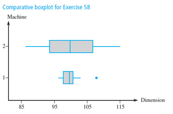
A company utilizes two different machines to manufacture parts of a certain type. During a single shift, a sample of n=20 parts produced by each machine is obtained, and the value of a particular critical dimension for each part is determined. The comparative boxplot at the bottom of this page is constructed from the resulting data. Compare and contrast the two samples.

See all solutions

Recommended explanations on Math Textbooks

View all explanations

What do you think about this solution?

We value your feedback to improve our textbook solutions.

Study anywhere. Anytime. Across all devices.