Explanations
  Textbooks
  Flashcards
  魅影直播 AI
  Notes
Notes  Study Plans
  Study Sets
  Find a degree
  Magazine
 Chapter 1: Q27E (page 28)
The article 鈥淪tudy on the Life Distribution of Microdrills鈥� (J. of Engr. Manufacture, 2002: 301鈥� 305) reported the following observations, listed in increasing order, on drill lifetime (number of holes that a drill machines before it breaks) when holes were drilled in a certain brass alloy.
11 14 20 23 31 36 39 44 47 50
59 61 65 67 68 71 74 76 78 79
81 84 85 89 91 93 96 99 101 104
105 105 112 118 123 136 139 141 148 158
161 168 184 206 248 263 289 322 388 513
a. Why can a frequency distribution not be based on the class intervals 0鈥�50, 50鈥�100, 100鈥�150, and so on?
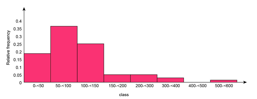
b. Construct a frequency distribution and histogram of the data using class boundaries 0, 50, 100, 鈥� , and then comment on interesting characteristics.
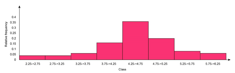
c. Construct a frequency distribution and histogram of the natural logarithms of the lifetime observations, and comment on interesting characteristics.
d. What proportion of the lifetime observations in this sample are less than 100? What proportion of the observations are at least 200?
Short Answer
a.
Observation 50 falls on a class boundary.
b. The histogram is represented as,
c. The histogram is represented as,
d.
The proportion of the lifetime observations in this sample that are less than 100 is 0.56.
The proportion of the lifetime observations in this sample that are at least200 is 0.14.
Step by step solution
Given information
The data for the drill lifetime (number of holes that a drill machines before it breaks) when holes were drilled in a certain brass alloy is provided.
Explain why frequency distribution for interval 0-50, 50-100 can not be constructed.
a.
The frequency distribution based on the class intervals 0-50, 50-100 cannot be constructed because the observation 50 falls on a class boundary.
Given information
The data for the drill lifetime (number of holes that a drill machines before it breaks) when holes were drilled in a certain brass alloy is provided.
Construct a frequency distribution and a histogram
b.
The relative frequency is computed as,
\({\rm{relative frequency }} = \frac{{frequency}}{{Total\;number\;of\;observations}}\)
The frequency distribution using the class boundaries 0,50,100 is as follows,
Class | Frequency | Relative frequency |
0鈭�&濒迟;50 | 9 | 0.18 |
50鈭�&濒迟;100 | 19 | 0.38 |
100鈭�&濒迟;150 | 11 | 0.22 |
150-<200 | 4 | 0.08 |
200鈭�&濒迟;300 | 4 | 0.08 |
300鈭�&濒迟;400 | 2 | 0.04 |
400鈭�&濒迟;500 | 0 | 0 |
500鈭�&濒迟;600 | 1 | 0.02 |
Total | 50 | 1 |
Steps to construct a histogram are,
1) Determine the frequency or the relative frequency.
2) Mark the class boundaries on the horizontal axis.
3) Draw a rectangle on the horizontal axis corresponding to the frequency or relative frequency.
The histogram is represented as,
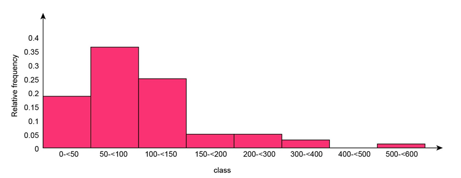
It can be observed from the above histogram that the distribution is positively skewed and the outliers are in the range of 500 to 600.
Given information
The data for the drill lifetime (number of holes that a drill machines before it breaks) when holes were drilled in a certain brass alloy is provided.
Construct a frequency distribution and a histogram
c.
The relative frequency is computed as,
\({\rm{relative frequency }} = \frac{{frequency}}{{Total\;number\;of\;observations}}\)
The frequency distribution of the natural logarithms of the lifetime observations is represented as,
Class | Frequency | Relative frequency |
2.25鈭�&濒迟;2.75 | 2 | 0.04 |
2.75鈭�&濒迟;3.25 | 2 | 0.04 |
3.25鈭�&濒迟;3.75 | 3 | 0.06 |
3.75鈭�&濒迟;4.25 | 8 | 0.16 |
4.25鈭�&濒迟;4.75 | 18 | 0.36 |
4.75鈭�&濒迟;5.25 | 10 | 0.2 |
5.25鈭�&濒迟;5.75 | 4 | 0.08 |
5.75鈭�&濒迟;6.25 | 3 | 0.06 |
Total | 50 | 1 |
Steps to construct a histogram are,
1) Determine the frequency or the relative frequency.
2) Mark the class boundaries on the horizontal axis.
3) Draw a rectangle on the horizontal axis corresponding to the frequency or relative frequency.
The histogram is represented as,
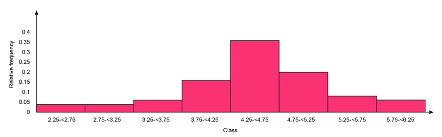
The characteristics of the above graph are:
1) The distribution is negatively skewed.
2) There are no outliers present.
3) The typical value is 4.25.
Given information
The data for the drill lifetime (number of holes that a drill machines before it breaks) when holes were drilled in a certain brass alloy is provided.
Compute the proportion
Referring to the relative frequencies computed in part b,
d.
Let x represents the drill lifetime.
The proportion of the lifetime observations in this sample that are less than 100 is computed as,
\(\begin{aligned}P\left( {x < 100} \right) &= P\left( {0 - < 50} \right) + P\left( {50 - < 100} \right)\\ &= 0.18 + 0.38\\ &= 0.56\end{aligned}\)
Thus, the proportion of the lifetime observations in this sample that are less than 100 is 0.56.
The proportion of the lifetime observations in this sample that are at least200 is computed as,
\(\begin{aligned}P\left( {x \ge 200} \right) &= 1 - \left( {P\left( {0 - < 50} \right) + P\left( {50 - < 100} \right) + P\left( {50 - < 150} \right) + P\left( {150 - < 200} \right)} \right)\\ &= 1 - \left( {0.18 + 0.38 + 0.22 + 0.08} \right)\\ &= 1 - 0.86\\ &= 0.14\end{aligned}\)
Thus, the proportion of the lifetime observations in this sample that are at least200 is 0.14.

Over 30 million students worldwide already upgrade their learning with 魅影直播!