
 Explanations
  Textbooks
  Flashcards
  魅影直播 AI
  Notes
Notes  Study Plans
  Study Sets
  Find a degree
  Magazine
 Chapter 1: Q19E (page 25)
The number of contaminating particles on a silicon waferprior to a certain rinsing process was determined for eachwafer in a sample of size 100, resulting in the followingfrequencies:
Number of particles 0 1 2 3 4 5 6 7
Frequency1 2 3 12 11 15 18 10
Number of particles8 9 10 11 12 13 14
Frequency12 4 5 3 1 2 1
a. What proportion of the sampled wafers had at leastone particle? At least five particles?
b. What proportion of the sampled wafers had betweenfive and ten particles, inclusive? Strictly between fiveand ten particles?
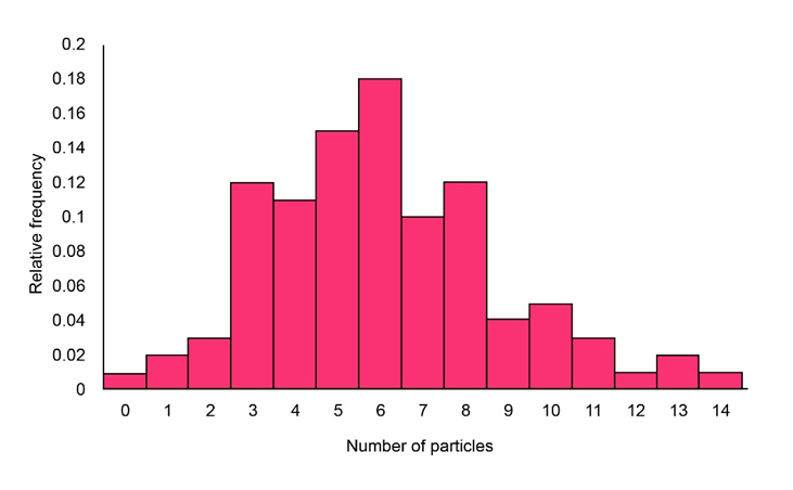
c. Draw a histogram using relative frequency on thevertical axis. How would you describe the shape of thehistogram?
Short Answer
a.The proportion of the sampled wafers that had at least one particle is 0.99.
The proportion of the sampled wafers that had at least five particlesis 0.71.
b.The proportion of the sampled wafers that had between five and ten particles, inclusive is 0.64.
The proportion of the sampled wafers that had between five and ten particles, strictlyis 0.44.
c.
Step by step solution
Given information
Thefrequencies of the number of contaminating particles on a silicon wafer prior to a certain rinsing processare provided.
The size of the sample is 100.
Calculate the proportion
Let X represents the number of particles.
The relative frequency is computed as,
\({\rm{relative frequency }} = \frac{{frequency}}{{Total\;number\;of\;observations}}\)
The table representing the relative frequency is computed as,
Number of particles | Frequency | Relative Frequency |
0 | 1 | 0.01 |
1 | 2 | 0.02 |
2 | 3 | 0.03 |
3 | 12 | 0.12 |
4 | 11 | 0.11 |
5 | 15 | 0.15 |
6 | 18 | 0.18 |
7 | 10 | 0.1 |
8 | 12 | 0.12 |
9 | 4 | 0.04 |
10 | 5 | 0.05 |
11 | 3 | 0.03 |
12 | 1 | 0.01 |
13 | 2 | 0.02 |
14 | 1 | 0.01 |
a.
Theproportion of the sampled wafers that had at least one particle is computed as,
\(\begin{aligned}P\left( {X \ge 1} \right) &= 1 - P\left( {X < 1} \right)\\ &= 1 - P\left( {X = 0} \right)\\ &= 1 - 0.01\\ &= 0.99\end{aligned}\)
Therefore, the proportion of the sampled wafers that had at least one particle is0.99.
The proportion of the sampled wafers that had at least five particlesis computed as,
\(\begin{aligned}P\left( {X \ge 5} \right) &= 1 - P\left( {X < 5} \right)\\ &= 1 - \left( {P\left( {X = 0} \right) + P\left( {X = 1} \right) + ... + P\left( {X = 4} \right)} \right)\\ &= 1 - \left( {0.01 + 0.02 + ... + 0.11} \right)\\ &= 1 - 0.29\\ &= 0.71\end{aligned}\)
Therefore, the proportion of the sampled wafers that had at least five particlesis 0.71.
Given information
Thefrequencies of the number of contaminating particles on a silicon wafer prior to a certain rinsing process are provided.
The size of the sample is 100.
Calculate the proportion
Let X represents the number of particles.
Referring to the relative frequencies of part a,
b.
Theproportion of the sampled wafers that had between five and ten particles, inclusive is computed as,
\(\begin{aligned}P\left( {5 \le X \le 10} \right) &= P\left( {X = 5} \right) + P\left( {X = 6} \right) + P\left( {X = 7} \right) + ... + P\left( {X = 10} \right)\\ &= 0.15 + 0.18 + 0.1 + ... + 0.05\\ &= 0.64\end{aligned}\)
Therefore, the proportion of the sampled wafers that had between five and ten particles, inclusive is 0.64.
Theproportion of the sampled wafers that had between five and ten particles, inclusive is computed as,
\(\begin{aligned}P\left( {5 < X < 10} \right) &= P\left( {X = 6} \right) + P\left( {X = 7} \right) + ... + P\left( {X = 9} \right)\\ &= 0.18 + 0.1 + ... + 0.01\\ &= 0.44\end{aligned}\)
Therefore, the proportion of the sampled wafers that had between five and ten particles, strictlyis 0.44.
Given information
Thefrequencies of the number of contaminating particles on a silicon wafer prior to a certain rinsing process are provided.
The size of the sample is 100.
Construct a histogram and comment on the shape
Referring to the relative frequencies computed in part a,
Steps to construct a histogram are,
1) Determine the frequency or the relative frequency.
2) Mark the class boundaries on the horizontal axis.
3) Draw a rectangle on the horizontal axis corresponding to the frequency or relative frequency.
The histogram is represented as,
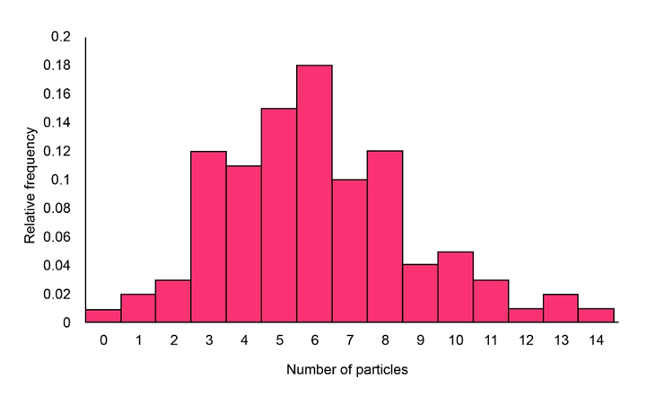
From the above-represented Histogram, it can be observed that it is close to moderate positive skewed.
Therefore, the shape is close to positive skewed.

Over 30 million students worldwide already upgrade their learning with 魅影直播!

