Chapter 5: Q13E (page 211)
You have two lightbulbs for a particular lamp. Let\({\rm{X = }}\)the lifetime of the first bulb and\({\rm{Y = }}\)the lifetime of the second bulb (both in\({\rm{1000}}\)s of hours). Suppose that\({\rm{X}}\)and\({\rm{Y}}\)are independent and that each has an exponential distribution with parameter\({\rm{\lambda = 1}}\).
a. What is the joint pdf of\({\rm{X}}\)and\({\rm{Y}}\)?
b. What is the probability that each bulb lasts at most\({\rm{1000}}\)hours (i.e.,\({\rm{X£1}}\)and\({\rm{Y£1)}}\)?
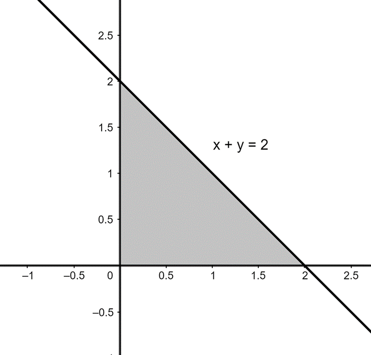
c. What is the probability that the total lifetime of the two bulbs is at most\({\rm{2}}\)? (Hint: Draw a picture of the region before integrating.)
d. What is the probability that the total lifetime is between\({\rm{1}}\)and\({\rm{2}}\)?
Short Answer
a) The joint pdf of X and Y is
b) The probability is \({\rm{P(X£1 and Y£1) = 0}}{\rm{.4}}\)
c) The probability is \({\rm{P(X + Y£2) = 0}}{\rm{.594}}\)
d) The probability is \({\rm{P(1£X + Y£2) = 0}}{\rm{.33}}\)
Step by step solution
Definition
Probability simply refers to the likelihood of something occurring. We may talk about the probabilities of particular outcomes—how likely they are—when we're unclear about the result of an event. Statistics is the study of occurrences guided by probability.
Step 2: The joint pdf of X and Y
Random variable \({\rm{X}}\) with pdf
is said to have exponential distribution with parameter\({\rm{\lambda }}\).
Therefore, we have
and
(a):
Two random variables \({\rm{X}}\) and \({\rm{Y}}\) are independent if and only if
1.\({\rm{p(x,y) = }}{{\rm{p}}_{\rm{X}}}{\rm{(x) \times }}{{\rm{p}}_{\rm{Y}}}{\rm{(y)}}\), for every \({\rm{(x,y)}}\) and when \({\rm{X}}\) and \({\rm{Y}}\) discrete rv's,
2.\({\rm{f(x,y) = }}{{\rm{f}}_{\rm{X}}}{\rm{(x) \times }}{{\rm{f}}_{\rm{Y}}}{\rm{(y)}}\), for every \({\rm{(x,y)}}\) and when \({\rm{X}}\) and \({\rm{Y}}\) continuous rv's, otherwise they are dependent.
We are given that random variables \({\rm{X}}\) and \({\rm{Y}}\) are independent, therefore, the joint pdf of \({\rm{X}}\) and \({\rm{Y}}\) is
Step 3: Calculating the probability
(b):
As given in the hints, the following is true
\(\begin{aligned}{l}{\rm{P(X£1 and Y£1)}}\mathop {\rm{ = }}\limits^{{\rm{(1)}}} {\rm{P(X£1) \times P(Y£1)}}\\\mathop {\rm{ = }}\limits^{{\rm{(2)}}} \left( {{\rm{1 - }}{{\rm{e}}^{{\rm{ - 1}}}}} \right){\rm{ \times }}\left( {{\rm{1 - }}{{\rm{e}}^{{\rm{ - 1}}}}} \right)\\{\rm{ = 0}}{\rm{.4}}\end{aligned}\)
(1): from the multiplication property given below,
(2): cof of exponentially distributed random variable is
Multiplication Property: Two events A and B are independent if and only if
\({\rm{P(A\c{C}B) = P(A) \times P(B)}}\)
Step 4: Calculating the probability
(c):
From the picture we can notice over what area should we integrate (the shaded area). Hence,
\(\begin{aligned}{\rm{P(X + Y£2)}}\mathop {\rm{ = }}\limits^{{\rm{(1)}}} \int_{\rm{0}}^{\rm{2}} {\int_{\rm{0}}^{{\rm{2 - x}}} {{{\rm{e}}^{{\rm{ - x - y}}}}} } {\rm{dydx}}\\{\rm{ = }}\int_{\rm{0}}^{\rm{2}} {\int_{\rm{0}}^{{\rm{2 - x}}} {{{\rm{e}}^{{\rm{ - x}}}}} } {{\rm{e}}^{{\rm{ - y}}}}{\rm{dydx}}\\{\rm{ = }}\int_{\rm{0}}^{\rm{2}} {{{\rm{e}}^{{\rm{ - x}}}}} \left( {{\rm{ - }}\left. {{{\rm{e}}^{{\rm{ - y}}}}} \right|_{\rm{0}}^{{\rm{2 - x}}}} \right){\rm{dx}}\\{\rm{ = }}\int_{\rm{0}}^{\rm{2}} {{{\rm{e}}^{{\rm{ - x}}}}} \left( {{\rm{1 - }}{{\rm{e}}^{{\rm{x - 2}}}}} \right){\rm{dx}}\\{\rm{ = }}\int_{\rm{0}}^{\rm{2}} {{{\rm{e}}^{{\rm{ - x}}}}} {\rm{dx - }}\int_{\rm{0}}^{\rm{2}} {{{\rm{e}}^{{\rm{ - 2}}}}} {\rm{dx}}\\{\rm{ = - }}\left. {{{\rm{e}}^{{\rm{ - x}}}}} \right|_{\rm{0}}^{\rm{2}}{\rm{ - 2}}{{\rm{e}}^{{\rm{ - 2}}}}\\{\rm{ = 1 - }}{{\rm{e}}^{{\rm{ - 2}}}}{\rm{ - 2}}{{\rm{e}}^{{\rm{ - 2}}}}\\{\rm{ = 0}}{\rm{.594}}\end{aligned}\)
(1): for every adequate set \({\rm{A}}\) the following holds
Step 5: Calculating the probability
d)
The following is true
\(\begin{aligned}{\rm{P(1£X + Y£2) = P(X + Y£2) - P(X + Y£1)}}\\\mathop {\rm{ = }}\limits^{{\rm{(1)}}} {\rm{0}}{\rm{.594 - 0}}{\rm{.264}}\\{\rm{ = 0}}{\rm{.33}}\end{aligned}\)
(1): the first probability has been calculated. The second probability can be calculated the same way as the first, we get
\(\begin{aligned}{\rm{P(X + Y£1) = }}\int_{\rm{0}}^{\rm{1}} {\int_{\rm{0}}^{{\rm{1 - x}}} {{{\rm{e}}^{{\rm{ - x - y}}}}} } {\rm{dydx}}\\{\rm{ = }}\int_{\rm{0}}^{\rm{1}} {\int_{\rm{0}}^{{\rm{1 - x}}} {{{\rm{e}}^{{\rm{ - x}}}}} } {{\rm{e}}^{{\rm{ - y}}}}{\rm{dydx}}\\{\rm{ = }}\int_{\rm{0}}^{\rm{1}} {{{\rm{e}}^{{\rm{ - x}}}}} \left( {{\rm{ - }}\left. {{{\rm{e}}^{{\rm{ - y}}}}} \right|_{\rm{0}}^{{\rm{1 - x}}}} \right){\rm{dx}}\\{\rm{ = }}\int_{\rm{0}}^{\rm{1}} {{{\rm{e}}^{{\rm{ - x}}}}} \left( {{\rm{1 - }}{{\rm{e}}^{{\rm{x - 1}}}}} \right){\rm{dx}}\\{\rm{ = }}\int_{\rm{0}}^{\rm{1}} {{{\rm{e}}^{{\rm{ - x}}}}} {\rm{dx - }}\int_{\rm{0}}^{\rm{1}} {{{\rm{e}}^{{\rm{ - 1}}}}} {\rm{dx}}\\{\rm{ = - }}\left. {{{\rm{e}}^{{\rm{ - x}}}}} \right|_{\rm{0}}^{\rm{1}}{\rm{ - }}{{\rm{e}}^{{\rm{ - 1}}}}\\{\rm{ = 1 - }}{{\rm{e}}^{{\rm{ - 1}}}}{\rm{ - }}{{\rm{e}}^{{\rm{ - 1}}}}\\{\rm{ = 0}}{\rm{.264}}{\rm{.}}\end{aligned}\)
Over 30 million students worldwide already upgrade their learning with ��Ӱֱ��!