/*! This file is auto-generated */ .wp-block-button__link{color:#fff;background-color:#32373c;border-radius:9999px;box-shadow:none;text-decoration:none;padding:calc(.667em + 2px) calc(1.333em + 2px);font-size:1.125em}.wp-block-file__button{background:#32373c;color:#fff;text-decoration:none} Q7E a. A random sample of 10 houses ... [FREE SOLUTION] | 魅影直播

魅影直播

a. A random sample of 10 houses in a particular area, each of which is heated with natural gas, is selected and the amount of gas (therms) used during the month of January is determined for each house. The resulting observations are 103, 156, 118, 89, 125, 147, 122, 109, 138, 99. Let m denote the average gas usage during January by all houses in this area. Compute a point estimate of m. b. Suppose there are 10,000 houses in this area that use natural gas for heating. Let t denote the total amount of gas used by all of these houses during January. Estimate t using the data of part (a). What estimator did you use in computing your estimate? c. Use the data in part (a) to estimate p, the proportion of all houses that used at least 100 therms. d. Give a point estimate of the population median usage (the middle value in the population of all houses) based on the sample of part (a). What estimator did you use?

Short Answer

Expert verified

a.The mean value is \({\rm{120}}{\rm{.6}}\).

b.Using the estimate from (a) for \(\mu \)we get \({\rm{1,206,000}}\).

c.The estimate of the proportion is \({\rm{0}}{\rm{.8}}\).

d.The sample median is average of the two mentioned values, is \ ({\rm{120}}\).

Step by step solution

01

Concept introduction

The standard deviation (SD) is a measure of the variability, or dispersion, between individual data values and the mean, whereas the standard error of the mean (SEM) is a measure of how far the sample mean (average) of the data is expected to differ from the genuine population mean. Always, the SEM is smaller than the SD.

02

Observing the sample mean

a.

The Sample Mean \(\bar x\) of observations \({x_1},{x_2}, \ldots ,{x_n}\)is given by

\(\begin{array}{c}\bar x = \frac{{{x_1} + {x_2} + \ldots + {x_n}}}{n}\\ = \frac{1}{n}\sum\limits_{i = 1}^n {{x_i}} \end{array}\)

The sample mean can be used for the point estimate of the mean value \((\mu )\)

\(\begin{array}{c}{\rm{\bar x = }}\frac{{{{\rm{x}}_{\rm{1}}}{\rm{ + }}{{\rm{x}}_{\rm{2}}}{\rm{ + \ldots + }}{{\rm{x}}_{\rm{n}}}}}{{\rm{n}}}\\{\rm{ = }}\frac{{\rm{1}}}{{{\rm{10}}}}{\rm{(103 + 156 + \ldots + 99)}}\\{\rm{ = }}\frac{{\rm{1}}}{{{\rm{10}}}}{\rm{ \times 1206}}\\{\rm{ = 120}}{\rm{.6}}\end{array}\)

Hence, the mean value is \({\rm{120}}{\rm{.6}}\).

03

Calculating part (b)

(b)

There are \({\rm{N = 10,000}}\)residences in the neighborhood. The total amount of gas used, \(\tau \), may be calculated with the help of the estimator .

\({\rm{\hat \tau = N \times \hat \mu }}\)

Using the estimate from (a) for \(\mu \)we get

\(\begin{array}{c}{\rm{\hat \tau = 10,000 \times 120}}{\rm{.6}}\\{\rm{ = 1,206,000}}\end{array}\)

Hence, using the estimate from (a) for \(\mu \)we get \({\rm{1,206,000}}\).

04

Finding estimate proportion

(c)

Because eight out of ten values in the given data are less than one hundred, the estimate of the proportion of all households that used at least one hundred terms is

\(\begin{array}{c}{\rm{\hat p = }}\frac{{\rm{8}}}{{{\rm{10}}}}\\{\rm{ = 0}}{\rm{.8}}\end{array}\)

Thus, the estimate of the proportion is \({\rm{0}}{\rm{.8}}\).

05

Estimating sample Median

(d)

The sample median can be used to get the median point estimate.

To begin, arrange the data in the following order:

\({\rm{89,99,103,109,118,122,125,138,147,156 }}\)

Because this sample has an even number of \({\rm{n = 10}}\)observations, the values of interest are.

\(\begin{array}{c}{\left( {\frac{{\rm{n}}}{{\rm{2}}}} \right)^{{\rm{th}}}}{\rm{ = }}{\left( {\frac{{{\rm{10}}}}{{\rm{2}}}} \right)^{{\rm{th}}}}\\{\rm{ = }}{{\rm{5}}^{{\rm{th}}}}\end{array}\)

where the \({5^{th}}\)and \({6^{th}}\)values are marked red in the ordered sample data. The sample median is average of the two mentioned values, hence

\(\begin{array}{c}{\rm{\tilde x = }}\frac{{{\rm{118 + 122}}}}{{\rm{2}}}\\{\rm{ = 120}}\end{array}\)

Therefore, the sample median is average of the two mentioned values, is \({\rm{120}}\)

Unlock Step-by-Step Solutions & Ace Your Exams!

  • Full Textbook Solutions

    Get detailed explanations and key concepts

  • Unlimited Al creation

    Al flashcards, explanations, exams and more...

  • Ads-free access

    To over 500 millions flashcards

  • Money-back guarantee

    We refund you if you fail your exam.

Over 30 million students worldwide already upgrade their learning with 魅影直播!

One App. One Place for Learning.

All the tools & learning materials you need for study success - in one app.

Get started for free

Most popular questions from this chapter

At time \({\rm{t = 0}}\), there is one individual alive in a certain population. A pure birth process then unfolds as follows. The time until the first birth is exponentially distributed with parameter \({\rm{\lambda }}\). After the first birth, there are two individuals alive. The time until the first gives birth again is exponential with parameter \({\rm{\lambda }}\), and similarly for the second individual. Therefore, the time until the next birth is the minimum of two exponential (\({\rm{\lambda }}\)) variables, which is exponential with parameter \({\rm{2\lambda }}\). Similarly, once the second birth has occurred, there are three individuals alive, so the time until the next birth is an exponential \({\rm{rv}}\) with parameter \({\rm{3\lambda }}\), and so on (the memoryless property of the exponential distribution is being used here). Suppose the process is observed until the sixth birth has occurred and the successive birth times are \({\rm{25}}{\rm{.2,41}}{\rm{.7,51}}{\rm{.2,55}}{\rm{.5,59}}{\rm{.5,61}}{\rm{.8}}\) (from which you should calculate the times between successive births). Derive the mle of l. (Hint: The likelihood is a product of exponential terms.)

Of \({{\rm{n}}_{\rm{1}}}\)randomly selected male smokers, \({{\rm{X}}_{\rm{1}}}\) smoked filter cigarettes, whereas of \({{\rm{n}}_{\rm{2}}}\) randomly selected female smokers, \({{\rm{X}}_{\rm{2}}}\) smoked filter cigarettes. Let \({{\rm{p}}_{\rm{1}}}\) and \({{\rm{p}}_{\rm{2}}}\) denote the probabilities that a randomly selected male and female, respectively, smoke filter cigarettes.

a. Show that \({\rm{(}}{{\rm{X}}_{\rm{1}}}{\rm{/}}{{\rm{n}}_{\rm{1}}}{\rm{) - (}}{{\rm{X}}_{\rm{2}}}{\rm{/}}{{\rm{n}}_{\rm{2}}}{\rm{)}}\) is an unbiased estimator for \({{\rm{p}}_{\rm{1}}}{\rm{ - }}{{\rm{p}}_{\rm{2}}}\). (Hint: \({\rm{E(}}{{\rm{X}}_{\rm{i}}}{\rm{) = }}{{\rm{n}}_{\rm{i}}}{{\rm{p}}_{\rm{i}}}\) for \({\rm{i = 1,2}}\).)

b. What is the standard error of the estimator in part (a)?

c. How would you use the observed values \({{\rm{x}}_{\rm{1}}}\) and \({{\rm{x}}_{\rm{2}}}\) to estimate the standard error of your estimator?

d. If \({{\rm{n}}_{\rm{1}}}{\rm{ = }}{{\rm{n}}_{\rm{2}}}{\rm{ = 200, }}{{\rm{x}}_{\rm{1}}}{\rm{ = 127}}\), and \({{\rm{x}}_{\rm{2}}}{\rm{ = 176}}\), use the estimator of part (a) to obtain an estimate of \({{\rm{p}}_{\rm{1}}}{\rm{ - }}{{\rm{p}}_{\rm{2}}}\).

e. Use the result of part (c) and the data of part (d) to estimate the standard error of the estimator.

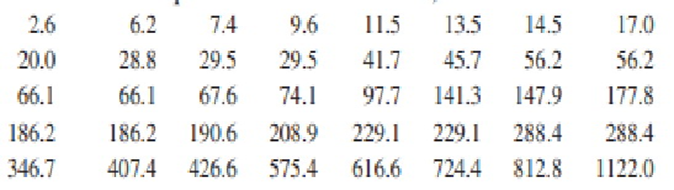
Urinary angiotensinogen (AGT) level is one quantitative indicator of kidney function. The article 鈥淯rinary Angiotensinogen as a Potential Biomarker of Chronic Kidney Diseases鈥 (J. of the Amer. Society of Hypertension, \({\rm{2008: 349 - 354}}\)) describes a study in which urinary AGT level \({\rm{(\mu g)}}\) was determined for a sample of adults with chronic kidney disease. Here is representative data (consistent with summary quantities and descriptions in the cited article):

An appropriate probability plot supports the use of the lognormal distribution (see Section \({\rm{4}}{\rm{.5}}\)) as a reasonable model for urinary AGT level (this is what the investigators did).

a. Estimate the parameters of the distribution. (Hint: Rem ember that \({\rm{X}}\) has a lognormal distribution with parameters \({\rm{\mu }}\) and \({{\rm{\sigma }}^{\rm{2}}}\) if \({\rm{ln(X)}}\) is normally distributed with mean \({\rm{\mu }}\) and variance \({{\rm{\sigma }}^{\rm{2}}}\).)

b. Use the estimates of part (a) to calculate an estimate of the expected value of AGT level. (Hint: What is \({\rm{E(X)}}\)?)

At time \({\rm{t = 0, 20}}\) identical components are tested. The lifetime distribution of each is exponential with parameter \({\rm{\lambda }}\). The experimenter then leaves the test facility unmonitored. On his return \({\rm{24}}\) hours later, the experimenter immediately terminates the test after noticing that \({\rm{y = 15}}\) of the \({\rm{20}}\) components are still in operation (so \({\rm{5}}\) have failed). Derive the mle of \({\rm{\lambda }}\). (Hint: Let \({\rm{Y = }}\) the number that survive \({\rm{24}}\) hours. Then \({\rm{Y}} \sim {\rm{Bin(n,p)}}\). What is the mle of \({\rm{p}}\)? Now notice that \({\rm{p = P(}}{{\rm{X}}_{\rm{i}}} \ge {\rm{24)}}\), where \({{\rm{X}}_{\rm{i}}}\) is exponentially distributed. This relates \({\rm{\lambda }}\) to \({\rm{p}}\), so the former can be estimated once the latter has been.)

\({{\rm{X}}_{\rm{1}}}{\rm{,}}.....{\rm{,}}{{\rm{X}}_{\rm{n}}}\)be a random sample from a gamma distribution with parameters \({\rm{\alpha }}\) and \({\rm{\beta }}\). a. Derive the equations whose solutions yield the maximum likelihood estimators of \({\rm{\alpha }}\) and \({\rm{\beta }}\). Do you think they can be solved explicitly? b. Show that the mle of \({\rm{\mu = \alpha \beta }}\) is \(\widehat {\rm{\mu }}{\rm{ = }}\overline {\rm{X}} \).

See all solutions

Recommended explanations on Math Textbooks

View all explanations

What do you think about this solution?

We value your feedback to improve our textbook solutions.

Study anywhere. Anytime. Across all devices.