/*! This file is auto-generated */ .wp-block-button__link{color:#fff;background-color:#32373c;border-radius:9999px;box-shadow:none;text-decoration:none;padding:calc(.667em + 2px) calc(1.333em + 2px);font-size:1.125em}.wp-block-file__button{background:#32373c;color:#fff;text-decoration:none} Q4E The article from which the data ... [FREE SOLUTION] | 魅影直播

魅影直播

The article from which the data in Exercise 1 was extracted also gave the accompanying strength observations for cylinders:

\(\begin{array}{l}\begin{array}{*{20}{r}}{{\rm{6}}{\rm{.1}}}&{{\rm{5}}{\rm{.8}}}&{{\rm{7}}{\rm{.8}}}&{{\rm{7}}{\rm{.1}}}&{{\rm{7}}{\rm{.2}}}&{{\rm{9}}{\rm{.2}}}&{{\rm{6}}{\rm{.6}}}&{{\rm{8}}{\rm{.3}}}&{{\rm{7}}{\rm{.0}}}&{{\rm{8}}{\rm{.3}}}\\{{\rm{7}}{\rm{.8}}}&{{\rm{8}}{\rm{.1}}}&{{\rm{7}}{\rm{.4}}}&{{\rm{8}}{\rm{.5}}}&{{\rm{8}}{\rm{.9}}}&{{\rm{9}}{\rm{.8}}}&{{\rm{9}}{\rm{.7}}}&{{\rm{14}}{\rm{.1}}}&{{\rm{12}}{\rm{.6}}}&{{\rm{11}}{\rm{.2}}}\end{array}\\\begin{array}{*{20}{l}}{{\rm{7}}{\rm{.8}}}&{{\rm{8}}{\rm{.1}}}&{{\rm{7}}{\rm{.4}}}&{{\rm{8}}{\rm{.5}}}&{{\rm{8}}{\rm{.9}}}&{{\rm{9}}{\rm{.8}}}&{{\rm{9}}{\rm{.7}}}&{{\rm{14}}{\rm{.1}}}&{{\rm{12}}{\rm{.6}}}&{{\rm{11}}{\rm{.2}}}\end{array}\end{array}\)

Prior to obtaining data, denote the beam strengths by X1, 鈥 ,Xm and the cylinder strengths by Y1, . . . , Yn. Suppose that the Xi 鈥檚 constitute a random sample from a distribution with mean m1 and standard deviation s1 and that the Yi 鈥檚 form a random sample (independent of the Xi 鈥檚) from another distribution with mean m2 and standard deviation\({{\rm{\sigma }}_{\rm{2}}}\).

a. Use rules of expected value to show that \({\rm{\bar X - \bar Y}}\)is an unbiased estimator of \({{\rm{\mu }}_{\rm{1}}}{\rm{ - }}{{\rm{\mu }}_{\rm{2}}}\). Calculate the estimate for the given data.

b. Use rules of variance from Chapter 5 to obtain an expression for the variance and standard deviation (standard error) of the estimator in part (a), and then compute the estimated standard error.

c. Calculate a point estimate of the ratio \({{\rm{\sigma }}_{\rm{1}}}{\rm{/}}{{\rm{\sigma }}_{\rm{2}}}\)of the two standard deviations.

d. Suppose a single beam and a single cylinder are randomly selected. Calculate a point estimate of the variance of the difference \({\rm{X - Y}}\) between beam strength and cylinder strength.

Short Answer

Expert verified

The estimate value is \({\rm{0}}{\rm{.434}}\)

The standard error is predicted to be \({\rm{0}}{\rm{.5687}}{\rm{.}}\)

The point estimate of the ratio \({\sigma _1}/{\sigma _2}\) is \(0.789\).

The point estimate of the variance is \({\rm{7}}{\rm{.1824}}\).

Step by step solution

01

Concept introduction

The mean of the sample mean X that we just calculated is identical to the population mean. We just calculated the standard deviation of the sample mean X, which is the population standard deviation divided by the square root of the sample size: 10=20/2.

02

Estimation of the sample mean for the beam strengths

(a)

The following holds,

\(\begin{array}{l}{\rm{E(\bar X - \bar Y) = E(\bar X) - E(\bar Y)}}\\{\rm{ = E}}\left( {\frac{{\rm{1}}}{{\rm{m}}}\sum\limits_{{\rm{i = 1}}}^{\rm{m}} {{{\rm{X}}_{\rm{i}}}} } \right){\rm{ - E}}\left( {\frac{{\rm{1}}}{{\rm{n}}}\sum\limits_{{\rm{n = 1}}}^{\rm{m}} {{{\rm{Y}}_{\rm{i}}}} } \right)\\{\rm{ = }}\frac{{\rm{1}}}{{\rm{m}}}\sum\limits_{{\rm{i = 1}}}^{\rm{m}} {\rm{E}} \left( {{{\rm{X}}_{\rm{i}}}} \right){\rm{ - }}\frac{{\rm{1}}}{{\rm{n}}}\sum\limits_{{\rm{i = 1}}}^{\rm{n}} {\rm{E}} \left( {{{\rm{Y}}_{\rm{i}}}} \right){\rm{n}}\\\mathop {\rm{ = }}\limits^{{\rm{(1)}}} \frac{{\rm{1}}}{{\rm{m}}}{\rm{ \times m \times E}}\left( {{{\rm{X}}_{\rm{1}}}} \right){\rm{ - }}\frac{{\rm{1}}}{{\rm{n}}}{\rm{ \times n \times E}}\left( {{{\rm{Y}}_{\rm{1}}}} \right)\\{\rm{ = }}{{\rm{\mu }}_{\rm{1}}}{\rm{ - }}{{\rm{\mu }}_{\rm{2}}}\end{array}\)

(1): The distributions of \({X_i}\)and \({Y_j}\)are identical.

This indicates that \(\bar X - \bar Y\)is an unbiased estimate of \({\mu _1} - {\mu _2}\).

The Sample Mean \(\bar x\)of observations \({x_1},{x_2}, \ldots ,{x_n}\)is calculated as follows:

\(\begin{array}{c}{\rm{\bar x = }}\frac{{{{\rm{x}}_{\rm{1}}}{\rm{ + }}{{\rm{x}}_{\rm{2}}}{\rm{ + \ldots + }}{{\rm{x}}_{\rm{n}}}}}{{\rm{n}}}\\{\rm{ = }}\frac{{\rm{1}}}{{\rm{n}}}\sum\limits_{{\rm{i = 1}}}^{\rm{n}} {{{\rm{x}}_{\rm{i}}}} \end{array}\)

The sample mean for the beam strengths data was calculated in exercise 1 and is barx=8.141. The sample mean for cylinder strengths is

\(\begin{array}{c}{\rm{\bar y = }}\frac{{\rm{1}}}{{{\rm{20}}}}{\rm{(6}}{\rm{.1 + 5}}{\rm{.8 + \ldots + 11}}{\rm{.12)}}\\{\rm{ = 8}}{\rm{.575}}\end{array}\)

Therefore, the estimate value is \(\begin{array}{c}{\rm{\bar x - \bar y = 8}}{\rm{.141 - 8}}{\rm{.575}}\\{\rm{ = 0}}{\rm{.434}}\end{array}\)

03

Calculation of standard deviation

(b)

The following is true for the variance due to independence:

\(\begin{array}{c}{\rm{V(\bar X - \bar Y)}}\mathop {\rm{ = }}\limits^{{\rm{(2)}}} {\rm{V(\bar X) + ( - 1}}{{\rm{)}}^{\rm{2}}}{\rm{V(\bar Y)}}\\{\rm{ = V}}\left( {\frac{{\rm{1}}}{{\rm{m}}}\sum\limits_{{\rm{i = 1}}}^{\rm{m}} {{{\rm{X}}_{\rm{i}}}} } \right){\rm{ + V}}\left( {\frac{{\rm{1}}}{{\rm{n}}}\sum\limits_{{\rm{n = 1}}}^{\rm{m}} {{{\rm{Y}}_{\rm{i}}}} } \right)\end{array}\)

\(\begin{array}{c}\mathop {\rm{ = }}\limits^{{\rm{(2)}}} \frac{{\rm{1}}}{{{{\rm{m}}^{\rm{2}}}}}\sum\limits_{{\rm{i = 1}}}^{\rm{m}} {\rm{V}} \left( {{{\rm{X}}_{\rm{i}}}} \right){\rm{ + }}\frac{{\rm{1}}}{{{{\rm{n}}^{\rm{2}}}}}\sum\limits_{{\rm{i = 1}}}^{\rm{n}} {\rm{V}} \left( {{{\rm{Y}}_{\rm{i}}}} \right)\\\mathop {\rm{ = }}\limits^{{\rm{(1)}}} \frac{{\rm{1}}}{{{{\rm{m}}^{\rm{2}}}}}{\rm{ \times m \times V}}\left( {{{\rm{X}}_{\rm{1}}}} \right){\rm{ + }}\frac{{\rm{1}}}{{{{\rm{n}}^{\rm{2}}}}}{\rm{ \times n \times V}}\left( {{{\rm{Y}}_{\rm{1}}}} \right)\\{\rm{ = }}\frac{{{\rm{\sigma }}_{\rm{1}}^{\rm{2}}}}{{\rm{m}}}{\rm{ + }}\frac{{{\rm{\sigma }}_{\rm{2}}^{\rm{2}}}}{{\rm{n}}}\end{array}\)

(2): Independence.

The standard deviation is

\(\begin{array}{l}{{\rm{\sigma }}_{{\rm{\bar X}}}}{\rm{ - \bar Y = }}\sqrt {{\rm{V(\bar X - \bar Y)}}} \\{\rm{ = }}\sqrt {\frac{{{\rm{\sigma }}_{\rm{1}}^{\rm{2}}}}{{\rm{m}}}{\rm{ + }}\frac{{{\rm{\sigma }}_{\rm{2}}^{\rm{2}}}}{{\rm{n}}}} \end{array}\)

The sample variances \(\sigma _1^2\)and \(\sigma _2^2\)are required in order to calculate the estimate. For the first time, the sample standard deviation was calculated.

\({{\rm{s}}_{\rm{1}}}{\rm{ = 1}}{\rm{.66}}\)

The Sample Variance is \({s^2}\)is\({s^2} = \frac{1}{{n - 1}} \cdot {S_{xx}}.\)

Where,

\(\begin{array}{c}{{\rm{S}}_{{\rm{xx}}}}{\rm{ = }}\sum {{{\left( {{{\rm{x}}_{\rm{i}}}{\rm{ - \bar x}}} \right)}^{\rm{2}}}} \\{\rm{ = }}\sum {{\rm{x}}_{\rm{i}}^{\rm{2}}} {\rm{ - }}\frac{{\rm{1}}}{{\rm{n}}}{\rm{ \times }}{\left( {\sum {{{\rm{x}}_{\rm{i}}}} } \right)^{\rm{2}}}\end{array}\)

The Sample Standard Deviation \({\rm{s}}\)is

\(\begin{array}{c}{\rm{s = }}\sqrt {{{\rm{s}}^{\rm{2}}}} \\{\rm{ = }}\sqrt {\frac{{\rm{1}}}{{{\rm{n - 1}}}}{\rm{ \times }}{{\rm{S}}_{{\rm{xx}}}}} \end{array}\)

The squared data points, \(y_i^2\),are

\(37.21,33.64,60.84,50.41,51.84,84.64,43.56,68.89,49,68.89,60.84,65.61,54.76,72.25,79.21,96.04,94.09,198.81,158.76,125.44,\)

Thus, the \({S_{yy}}\)is

\(\begin{array}{c}{{\rm{S}}_{{\rm{yy}}}}{\rm{ = }}\sum {{\rm{y}}_{\rm{i}}^{\rm{2}}} {\rm{ - }}\frac{{\rm{1}}}{{\rm{n}}}{\rm{ \times }}{\left( {\sum {{{\rm{y}}_{\rm{i}}}} } \right)^{\rm{2}}}\\{\rm{ = 37}}{\rm{.21 + 33}}{\rm{.64 + \ldots + 125}}{\rm{.44 - }}\frac{{\rm{1}}}{{{\rm{20}}}}{\rm{ \times (6}}{\rm{.1 + 5}}{\rm{.8 + \ldots + 11}}{\rm{.2}}{{\rm{)}}^{\rm{2}}}\\{\rm{ = 1554}}{\rm{.73 - }}\frac{{\rm{1}}}{{{\rm{16}}}}{\rm{ \times 171}}{\rm{.}}{{\rm{5}}^{\rm{2}}}\\{\rm{ = 84}}{\rm{.1175}}\end{array}\)

And the sample variance is

\(\begin{array}{c}{\rm{s}}_{\rm{2}}^{\rm{2}}{\rm{ = }}\frac{{\rm{1}}}{{{\rm{16 - 1}}}}{\rm{ \times 84}}{\rm{.1175}}\\{\rm{ = 4}}{\rm{.427}}\end{array}\)
Also, the sample standard deviation is

\(\begin{array}{c}{\rm{s = }}\sqrt {{{\rm{s}}^{\rm{2}}}} \\{\rm{ = }}\sqrt {{\rm{4}}{\rm{.427}}} \\{\rm{ = 2}}{\rm{.104}}{\rm{.}}\end{array}\)

As a result, the standard error is predicted to be \(\begin{array}{c}{{\rm{s}}_{{\rm{\bar X - \bar Y}}}}{\rm{ = }}\sqrt {\frac{{{\rm{s}}_{\rm{1}}^{\rm{2}}}}{{\rm{m}}}{\rm{ + }}\frac{{{\rm{s}}_{\rm{2}}^{\rm{2}}}}{{\rm{n}}}} \\{\rm{ = }}\sqrt {\frac{{{\rm{1}}{\rm{.6}}{{\rm{6}}^{\rm{2}}}}}{{{\rm{27}}}}{\rm{ + }}\frac{{{\rm{2}}{\rm{.10}}{{\rm{4}}^{\rm{2}}}}}{{{\rm{20}}}}} \\{\rm{ = 0}}{\rm{.5687}}{\rm{.}}\end{array}\)

Hence, the required result is\({\rm{0}}{\rm{.5687}}\).

04

Finding the point estimate of the ratio

(c)

The point estimate of the ratio \({\sigma _1}/{\sigma _2}\)

\(\begin{array}{c}\frac{{{s_1}}}{{{s_2}}} = \frac{{1.66}}{{2.104}}\\ = 0.789.\end{array}\)

Thus, the required result is\(0.789\).

05

Finding the point estimate of the variance

(d)

The variance of \(X - Y\)is

\(\begin{array}{c}{\rm{V(X - Y)}}\mathop {\rm{ = }}\limits^{{\rm{(2)}}} {\rm{V(X) + ( - 1}}{{\rm{)}}^{\rm{2}}}{\rm{V(Y)}}\\{\rm{ = \sigma }}_{\rm{1}}^{\rm{2}}{\rm{ + \sigma }}_{\rm{2}}^{\rm{2}}\end{array}\)

which yields a point estimate of the variance

\(\begin{array}{c}{\rm{s}}_{\rm{1}}^{\rm{2}}{\rm{ + s}}_{\rm{2}}^{\rm{2}}{\rm{ = 1}}{\rm{.6}}{{\rm{6}}^{\rm{2}}}{\rm{ + 2}}{\rm{.10}}{{\rm{4}}^{\rm{2}}}\\{\rm{ = 7}}{\rm{.1824}}\end{array}\)

Hence, the point estimate of the variance is\({\rm{7}}{\rm{.1824}}\).

Unlock Step-by-Step Solutions & Ace Your Exams!

  • Full Textbook Solutions

    Get detailed explanations and key concepts

  • Unlimited Al creation

    Al flashcards, explanations, exams and more...

  • Ads-free access

    To over 500 millions flashcards

  • Money-back guarantee

    We refund you if you fail your exam.

Over 30 million students worldwide already upgrade their learning with 魅影直播!

One App. One Place for Learning.

All the tools & learning materials you need for study success - in one app.

Get started for free

Most popular questions from this chapter

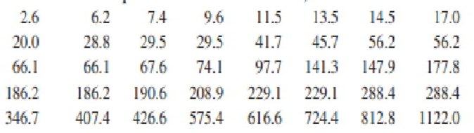
We defined a negative binomial\({\rm{rv}}\)as the number of failures that occur before the\({\rm{rth}}\)success in a sequence of independent and identical success/failure trials. The probability mass function (\({\rm{pmf}}\)) of\({\rm{X}}\)is\({\rm{nb(x,r,p) = }}\)\(\left( {\begin{array}{*{20}{c}}{{\rm{x + r - 1}}}\\{\rm{x}}\end{array}} \right){{\rm{p}}^{\rm{r}}}{{\rm{(1 - p)}}^{\rm{x}}}\quad {\rm{x = 0,1,2, \ldots }}\)

a. Suppose that. Show that\({\rm{\hat p = (r - 1)/(X + r - 1)}}\)is an unbiased estimator for\({\rm{p}}\). (Hint: Write out\({\rm{E(\hat p)}}\)and cancel\({\rm{x + r - 1}}\)inside the sum.)

b. A reporter wishing to interview five individuals who support a certain candidate begins asking people whether\({\rm{(S)}}\)or not\({\rm{(F)}}\)they support the candidate. If the sequence of responses is SFFSFFFSSS, estimate\({\rm{p = }}\)the true proportion who support the candidate.

A vehicle with a particular defect in its emission control system is taken to a succession of randomly selected mechanics until\({\rm{r = 3}}\)of them have correctly diagnosed the problem. Suppose that this requires diagnoses by\({\rm{20}}\)different mechanics (so there were\({\rm{17}}\)incorrect diagnoses). Let\({\rm{p = P}}\)(correct diagnosis), so\({\rm{p}}\)is the proportion of all mechanics who would correctly diagnose the problem. What is the mle of\({\rm{p}}\)? Is it the same as the mle if a random sample of\({\rm{20}}\)mechanics results in\({\rm{3}}\)correct diagnoses? Explain. How does the mle compare to the estimate resulting from the use of the unbiased estimator?

Let\({{\rm{X}}_{\rm{1}}}{\rm{,}}{{\rm{X}}_{\rm{2}}}{\rm{, \ldots ,}}{{\rm{X}}_{\rm{n}}}\)represent a random sample from a Rayleigh distribution with pdf

\({\rm{f(x,\theta ) = }}\frac{{\rm{x}}}{{\rm{\theta }}}{{\rm{e}}^{{\rm{ - }}{{\rm{x}}^{\rm{2}}}{\rm{/(2\theta )}}}}\quad {\rm{x > 0}}\)a. It can be shown that\({\rm{E}}\left( {{{\rm{X}}^{\rm{2}}}} \right){\rm{ = 2\theta }}\). Use this fact to construct an unbiased estimator of\({\rm{\theta }}\)based on\({\rm{\Sigma X}}_{\rm{i}}^{\rm{2}}\)(and use rules of expected value to show that it is unbiased).

b. Estimate\({\rm{\theta }}\)from the following\({\rm{n = 10}}\)observations on vibratory stress of a turbine blade under specified conditions:

\(\begin{array}{*{20}{l}}{{\rm{16}}{\rm{.88}}}&{{\rm{10}}{\rm{.23}}}&{{\rm{4}}{\rm{.59}}}&{{\rm{6}}{\rm{.66}}}&{{\rm{13}}{\rm{.68}}}\\{{\rm{14}}{\rm{.23}}}&{{\rm{19}}{\rm{.87}}}&{{\rm{9}}{\rm{.40}}}&{{\rm{6}}{\rm{.51}}}&{{\rm{10}}{\rm{.95}}}\end{array}\)

The shear strength of each of ten test spot welds is determined, yielding the following data (psi):

\(\begin{array}{*{20}{l}}{{\rm{392}}}&{{\rm{376}}}&{{\rm{401}}}&{{\rm{367}}}&{{\rm{389}}}&{{\rm{362}}}&{{\rm{409}}}&{{\rm{415}}}&{{\rm{358}}}&{{\rm{375}}}\end{array}\)

a. Assuming that shear strength is normally distributed, estimate the true average shear strength and standard deviation of shear strength using the method of maximum likelihood.

b. Again assuming a normal distribution, estimate the strength value below which\({\rm{95\% }}\)of all welds will have their strengths. (Hint: What is the\({\rm{95 th}}\)percentile in terms of\({\rm{\mu }}\)and\({\rm{\sigma }}\)? Now use the invariance principle.)

c. Suppose we decide to examine another test spot weld. Let\({\rm{X = }}\)shear strength of the weld. Use the given data to obtain the mle of\({\rm{P(X拢400)}}{\rm{.(Hint:P(X拢400) = \Phi ((400 - \mu )/\sigma )}}{\rm{.)}}\)

Urinary angiotensinogen (AGT) level is one quantitative indicator of kidney function. The article 鈥淯rinary Angiotensinogen as a Potential Biomarker of Chronic Kidney Diseases鈥 (J. of the Amer. Society of Hypertension, \({\rm{2008: 349 - 354}}\)) describes a study in which urinary AGT level \({\rm{(\mu g)}}\) was determined for a sample of adults with chronic kidney disease. Here is representative data (consistent with summary quantities and descriptions in the cited article):

An appropriate probability plot supports the use of the lognormal distribution (see Section \({\rm{4}}{\rm{.5}}\)) as a reasonable model for urinary AGT level (this is what the investigators did).

a. Estimate the parameters of the distribution. (Hint: Rem ember that \({\rm{X}}\) has a lognormal distribution with parameters \({\rm{\mu }}\) and \({{\rm{\sigma }}^{\rm{2}}}\) if \({\rm{ln(X)}}\) is normally distributed with mean \({\rm{\mu }}\) and variance \({{\rm{\sigma }}^{\rm{2}}}\).)

b. Use the estimates of part (a) to calculate an estimate of the expected value of AGT level. (Hint: What is \({\rm{E(X)}}\)?)

See all solutions

Recommended explanations on Math Textbooks

View all explanations

What do you think about this solution?

We value your feedback to improve our textbook solutions.

Study anywhere. Anytime. Across all devices.