/*! This file is auto-generated */ .wp-block-button__link{color:#fff;background-color:#32373c;border-radius:9999px;box-shadow:none;text-decoration:none;padding:calc(.667em + 2px) calc(1.333em + 2px);font-size:1.125em}.wp-block-file__button{background:#32373c;color:#fff;text-decoration:none} Q1E The accompanying data on flexura... [FREE SOLUTION] | 魅影直播

魅影直播

The accompanying data on flexural strength (MPa) for concrete beams of a certain type was introduced in Example 1.2.

\(\begin{array}{*{20}{r}}{{\rm{5}}{\rm{.9}}}&{{\rm{7}}{\rm{.2}}}&{{\rm{7}}{\rm{.3}}}&{{\rm{6}}{\rm{.3}}}&{{\rm{8}}{\rm{.1}}}&{{\rm{6}}{\rm{.8}}}&{{\rm{7}}{\rm{.0}}}\\{{\rm{7}}{\rm{.6}}}&{{\rm{6}}{\rm{.8}}}&{{\rm{6}}{\rm{.5}}}&{{\rm{7}}{\rm{.0}}}&{{\rm{6}}{\rm{.3}}}&{{\rm{7}}{\rm{.9}}}&{{\rm{9}}{\rm{.0}}}\\{{\rm{3}}{\rm{.2}}}&{{\rm{8}}{\rm{.7}}}&{{\rm{7}}{\rm{.8}}}&{{\rm{9}}{\rm{.7}}}&{{\rm{7}}{\rm{.4}}}&{{\rm{7}}{\rm{.7}}}&{{\rm{9}}{\rm{.7}}}\\{{\rm{7}}{\rm{.3}}}&{{\rm{7}}{\rm{.7}}}&{{\rm{11}}{\rm{.6}}}&{{\rm{11}}{\rm{.3}}}&{{\rm{11}}{\rm{.8}}}&{{\rm{10}}{\rm{.7}}}&{}\end{array}\)

Calculate a point estimate of the mean value of strength for the conceptual population of all beams manufactured in this fashion, and state which estimator you used\({\rm{(Hint:\Sigma }}{{\rm{x}}_{\rm{i}}}{\rm{ = 219}}{\rm{.8}}{\rm{.)}}\)

b. Calculate a point estimate of the strength value that separates the weakest 50% of all such beams from the strongest 50 %, and state which estimator you used.

c. Calculate and interpret a point estimate of the population standard deviation\({\rm{\sigma }}\). Which estimator did you use?\({\rm{(Hint:}}\left. {{\rm{\Sigma x}}_{\rm{i}}^{\rm{2}}{\rm{ = 1860}}{\rm{.94}}{\rm{.}}} \right)\)

d. Calculate a point estimate of the proportion of all such beams whose flexural strength exceeds\({\rm{10MPa}}\). (Hint: Think of an observation as a "success" if it exceeds 10.)

e. Calculate a point estimate of the population coefficient of variation\({\rm{\sigma /\mu }}\), and state which estimator you used.

Short Answer

Expert verified

a. \(8.1407,\)Sample mean.

b. \({\rm{7}}{\rm{.7,}}\) Sample mean.

c. \({\rm{1}}{\rm{.6595,}}\) Sample standard deviation.

d. \({\rm{0}}{\rm{.1481 }}\)of \({\rm{14}}{\rm{.81 \% ,}}\)Sample Proportion.

e. \({\rm{0}}{\rm{.2039 }}\)or \(20.39{\rm{ }}\% ,\)Sample coefficient of variation.

Step by step solution

01

Concept Introduction

We can compute probabilities with regard to means using Z scores because the sample means are normally distributed.

We used Z scores to compute probabilities for values among individuals in a population.

02

Step 2:Estimating of the mean value

(a)

Given,

\(\begin{array}{c}\sum {{{\rm{x}}_{\rm{i}}}} {\rm{ = 219}}{\rm{.8}}\\{\rm{n = 27}}\end{array}\)

The sample mean, which is the total of all values divided by the number of values, is the point estimate of the mean value:

\(\begin{array}{c}\bar x = \frac{{\sum {{x_i}} }}{n}\\ = \frac{{219.8}}{{27}}\\ \approx 8.1407\end{array}\)

Therefore, the estimate of the mean value is \(8.1407\)

03

Finding the Median Point

(b)

The median is the point estimate that divides the weakest \(50\% \)from the greatest \(50\% \).Sort the data values as follows:

\(\begin{array}{l}{\rm{5}}{\rm{.9,6}}{\rm{.3,6}}{\rm{.3,6}}{\rm{.5,6}}{\rm{.8,6}}{\rm{.8,7,7,7}}{\rm{.2,7}}{\rm{.3,7}}{\rm{.4,7}}{\rm{.6,7}}{\rm{.7,7}}{\rm{.7,7}}{\rm{.8,7}}{\rm{.8,7}}{\rm{.9,8}}{\rm{.1,8}}{\rm{.2,8}}{\rm{.7,9,9}}{\rm{.7,9}}{\rm{.7,10}}{\rm{.7,11}}{\rm{.3,11}}{\rm{.6,11}}{\rm{.8}}\\\end{array}\)

The median is the middle (14th data value) of the sorted data set, because there are 27 data values in the data set.

\({\rm{M = 7}}{\rm{.7}}\)

Hence, the Median point is \({\rm{M = 7}}{\rm{.7}}\)

04

Estimating of the population standard deviation.

(c)

Given:

\(\begin{array}{c}\sum {x_i^2} = 1860.94\\\sum {{x_i}} = 219.8\\n = 27\end{array}\)

The sample standard deviation is the point estimate of the population standard deviation.

\(\begin{aligned} s &= \sqrt {\frac{{\sum {{x^2}} - {{\left( {\sum x } \right)}^2}/n}}{{n - 1}}} \\ &= \sqrt {\frac{{1860.94 - {{(219.8)}^2}/27}}{{27 - 1}}} \\ \approx 1.6595\end{aligned}\)

As a result, the population standard deviation is \(1.6595\)

05

Calculating the sample proportion

(d)

The sample proportion is the point estimate of the proportion. The sample proportion is calculated by dividing the number of successes (values greater than 10) by the sample size \(n = 27:\)

\(\begin{array}{c}\hat p = \frac{4}{{27}}\\ \approx 0.1481\\ = 14.81\% \end{array}\)

Such that, the sample proportion is \(14.81\% \).

06

Estimating the population coefficient

(e)

The sample coefficient of variation \(s/\bar x\)is the point estimate of the population coefficient of variation \(\sigma /\mu \)

\(\begin{aligned}CV &= \frac{s}{{\bar x}}\\ &= \frac{{1.6595}}{{8.1407}}\\ \approx 0.2039\\ &= 20.39\% \end{aligned}\)

Therefore, the sample coefficient variation is \(20.39\% \).

Unlock Step-by-Step Solutions & Ace Your Exams!

  • Full Textbook Solutions

    Get detailed explanations and key concepts

  • Unlimited Al creation

    Al flashcards, explanations, exams and more...

  • Ads-free access

    To over 500 millions flashcards

  • Money-back guarantee

    We refund you if you fail your exam.

Over 30 million students worldwide already upgrade their learning with 魅影直播!

One App. One Place for Learning.

All the tools & learning materials you need for study success - in one app.

Get started for free

Most popular questions from this chapter

At time \({\rm{t = 0}}\), there is one individual alive in a certain population. A pure birth process then unfolds as follows. The time until the first birth is exponentially distributed with parameter \({\rm{\lambda }}\). After the first birth, there are two individuals alive. The time until the first gives birth again is exponential with parameter \({\rm{\lambda }}\), and similarly for the second individual. Therefore, the time until the next birth is the minimum of two exponential (\({\rm{\lambda }}\)) variables, which is exponential with parameter \({\rm{2\lambda }}\). Similarly, once the second birth has occurred, there are three individuals alive, so the time until the next birth is an exponential \({\rm{rv}}\) with parameter \({\rm{3\lambda }}\), and so on (the memoryless property of the exponential distribution is being used here). Suppose the process is observed until the sixth birth has occurred and the successive birth times are \({\rm{25}}{\rm{.2,41}}{\rm{.7,51}}{\rm{.2,55}}{\rm{.5,59}}{\rm{.5,61}}{\rm{.8}}\) (from which you should calculate the times between successive births). Derive the mle of l. (Hint: The likelihood is a product of exponential terms.)

Consider randomly selecting \({\rm{n}}\) segments of pipe and determining the corrosion loss (mm) in the wall thickness for each one. Denote these corrosion losses by \({{\rm{Y}}_{\rm{1}}}{\rm{,}}.....{\rm{,}}{{\rm{Y}}_{\rm{n}}}\). The article 鈥淎 Probabilistic Model for a Gas Explosion Due to Leakages in the Grey Cast Iron Gas Mains鈥 (Reliability Engr. and System Safety (\({\rm{(2013:270 - 279)}}\)) proposes a linear corrosion model: \({{\rm{Y}}_{\rm{i}}}{\rm{ = }}{{\rm{t}}_{\rm{i}}}{\rm{R}}\), where \({{\rm{t}}_{\rm{i}}}\) is the age of the pipe and \({\rm{R}}\), the corrosion rate, is exponentially distributed with parameter \({\rm{\lambda }}\). Obtain the maximum likelihood estimator of the exponential parameter (the resulting mle appears in the cited article). (Hint: If \({\rm{c > 0}}\) and \({\rm{X}}\) has an exponential distribution, so does \({\rm{cX}}\).)

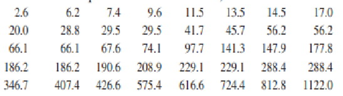
Urinary angiotensinogen (AGT) level is one quantitative indicator of kidney function. The article 鈥淯rinary Angiotensinogen as a Potential Biomarker of Chronic Kidney Diseases鈥 (J. of the Amer. Society of Hypertension, \({\rm{2008: 349 - 354}}\)) describes a study in which urinary AGT level \({\rm{(\mu g)}}\) was determined for a sample of adults with chronic kidney disease. Here is representative data (consistent with summary quantities and descriptions in the cited article):

An appropriate probability plot supports the use of the lognormal distribution (see Section \({\rm{4}}{\rm{.5}}\)) as a reasonable model for urinary AGT level (this is what the investigators did).

a. Estimate the parameters of the distribution. (Hint: Rem ember that \({\rm{X}}\) has a lognormal distribution with parameters \({\rm{\mu }}\) and \({{\rm{\sigma }}^{\rm{2}}}\) if \({\rm{ln(X)}}\) is normally distributed with mean \({\rm{\mu }}\) and variance \({{\rm{\sigma }}^{\rm{2}}}\).)

b. Use the estimates of part (a) to calculate an estimate of the expected value of AGT level. (Hint: What is \({\rm{E(X)}}\)?)

In a random sample of 80 components of a certain type, 12 are found to be defective.

a. Give a point estimate of the proportion of all such components that are not defective.

b. A system is to be constructed by randomly selecting two of these components and connecting them in series, as shown here.

The series connection implies that the system will function if and only if neither component is defective (i.e., both components work properly). Estimate the proportion of all such systems that work properly. (Hint: If p denotes the probability that a component works properly, how can P (system works) be expressed in terms of p ?)

A sample of \({\rm{n}}\) captured Pandemonium jet fighters results in serial numbers\({{\rm{x}}_{\rm{1}}}{\rm{,}}{{\rm{x}}_{\rm{2}}}{\rm{,}}{{\rm{x}}_{\rm{3}}}{\rm{, \ldots ,}}{{\rm{x}}_{\rm{n}}}\). The CIA knows that the aircraft were numbered consecutively at the factory starting with \({\rm{\alpha }}\)and ending with\({\rm{\beta }}\), so that the total number of planes manufactured is \({\rm{\beta - \alpha + 1}}\) (e.g., if \({\rm{\alpha = 17}}\) and\({\rm{\beta = 29}}\), then \({\rm{29 - 17 + 1 = 13}}\)planes having serial numbers \({\rm{17,18,19, \ldots ,28,29}}\)were manufactured). However, the CIA does not know the values of \({\rm{\alpha }}\) or\({\rm{\beta }}\). A CIA statistician suggests using the estimator \({\rm{max}}\left( {{{\rm{X}}_{\rm{i}}}} \right){\rm{ - min}}\left( {{{\rm{X}}_{\rm{i}}}} \right){\rm{ + 1}}\)to estimate the total number of planes manufactured.

a. If\({\rm{n = 5, x\_}}\left\{ {\rm{1}} \right\}{\rm{ = 237, x\_}}\left\{ {\rm{2}} \right\}{\rm{ = 375, x\_}}\left\{ {\rm{3}} \right\}{\rm{ = 202, x\_}}\left\{ {\rm{4}} \right\}{\rm{ = 525,}}\)and\({{\rm{x}}_{\rm{5}}}{\rm{ = 418}}\), what is the corresponding estimate?

b. Under what conditions on the sample will the value of the estimate be exactly equal to the true total number of planes? Will the estimate ever be larger than the true total? Do you think the estimator is unbiased for estimating\({\rm{\beta - \alpha + 1}}\)? Explain in one or two sentences.

See all solutions

Recommended explanations on Math Textbooks

View all explanations

What do you think about this solution?

We value your feedback to improve our textbook solutions.

Study anywhere. Anytime. Across all devices.