Explanations
  Textbooks
  Flashcards
  魅影直播 AI
  Notes
Notes  Study Plans
  Study Sets
  Find a degree
  Magazine
 Chapter 11: Q2E (page 448)
Four different coatings are being considered for corrosion protection of metal pipe. The pipe will be buried in three different types of soil. To investigate whether the amount of corrosion depends either on the coating or on the type of soil, 12 pieces of pipe are selected. Each piece is coated with one of the four coatings and buried in one of the three types of soil for a fixed time, after which the amount of corrosion (depth of maximum pits, in .0001 in.) is determined. The data appears in the table.
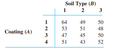
a. Assuming the validity of the additive model, carry out the ANOVA analysis using an ANOVA table to see whether the amount of corrosion depends on either the type of coating used or the type of soil. Use=.05.
b. Compute\(\hat \mu ,{\hat \alpha _1},{\hat \alpha _2},{\hat \alpha _3},{\hat \alpha _4},{\hat \beta _1},{\hat \beta _2},\;and\;{\hat \beta _3}\)
Short Answer
\(\begin{aligned}{l}{\rm{a}}{\rm{. Do not reject null hypotheses\;}}{H_{0A}}{\rm{\;and\;}}{H_{0B}}{\rm{. }}\\{\rm{b}}{\rm{. Estimate the value using the sample means}}{\rm{.\;}}\end{aligned}\)
Step by step solution
Determine the factors:
a)-
Let
Where the following holds
and where the are independent normally distributed random variable with mean 0 and varianceThe hypotheses of interest are
\({H_{0A}}:{\alpha _1} = {\alpha _2} = \ldots = {\alpha _I} = 0{\rm{\;versus\;}}{H_{aA}}:{\rm{\;at least one\;}}{\alpha _ - }i \ne 0\)
And for the factor B
\({H_{0B}}:{\beta _1} = {\beta _2} = \ldots = {\beta _J} = 0{\rm{\;versus\;}}{H_{aB}}:{\rm{\;at least one\;}}{\beta _ - }j \ne 0.{\rm{\;}}\)
Obtain the average of measurements:
The following table summarizes values which will be required to compute the test statistic value.
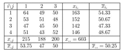
Values of I and J are
\(I = 4\)- number of rows;
J = 3 鈥� number of columns.
Before continuing, denote withthe average of measurements obtained when factor A is held at level i.
Withthe average of measurements obtained when factor B is held at level j
And with.. the grand mean
Observed values are denoted with small instead of big X. The notations without line over X are just the sums.
Determine average of measurements for factor B
Compute them one by one. Starting with average of measurements for factor A at level corresponding level
\(\begin{aligned}{*{20}{c}}{{x_{1.}} = 64 + 49 + 50 = 163}\\{{x_{2.}} = 53 + 51 + 48 = 152}\\{{x_{3.}} = 47 + 45 + 50 = 142}\\{{x_{4.}} = 51 + 43 + 52 = 146}\end{aligned}\)
Values of
\({\bar x_{i.}} = \frac{1}{J} \cdot {x_i}\)
Are given by
\(\begin{aligned}{*{20}{c}}{{{\bar x}_{1.}} = \frac{1}{3} \cdot 163 = 54.33}\\{{{\bar x}_{2.}} = \frac{1}{3} \cdot 152 = 50.67}\\{{{\bar x}_{3.}} = \frac{1}{3} \cdot 142 = 47.33}\\{{{\bar x}_{4.}} = \frac{1}{3} \cdot 146 = 48.67}\end{aligned}\)
The average of measurements for factor B at level corresponding level
\(\begin{aligned}{*{20}{c}}{{x_{.1}} = 64 + 53 + 47 + 51 = 215}\\{{x_{.2}} = 49 + 51 + 45 + 43 = 188}\\{{x_{.3}} = 50 + 48 + 50 + 52 = 200.}\end{aligned}\)
Values of
\({\bar x_{ \cdot j}} = \frac{1}{I} \cdot {x_{ \cdot j}}\)
Are given by
\(\begin{aligned}{*{20}{c}}{{{\bar x}_{.1}} = \frac{1}{4} \cdot 215 = 53.75;}\\{{{\bar x}_{.2}} = \frac{1}{4} \cdot 188 = 47;}\\{{{\bar x}_{.3}} = \frac{1}{4} \cdot 200 = 50.}\end{aligned}\)
Find the sum of squares:
The grand sum is
The grand mean is
The sum of squares are given by
with degrees of freedom respectively,
\(\begin{aligned}{*{20}{c}}{d{f_T} = IJ - 1}\\{d{f_A} = I - 1}\\{d{f_B} = J - 1}\\{d{f_E} = (I - 1)(J - 1).}\end{aligned}\)
SST can be computed as
SSA can be computed as
\(\begin{aligned}{*{20}{c}}{ = \frac{1}{3} \cdot \left( {{{163}^2} + {{152}^2} + {{142}^2} + {{146}^2}} \right) - \frac{1}{{4 \cdot 3}} \cdot {{603}^2}}\\{ = 30,384.33 - 30,300.75}\\{ = 83.58}\end{aligned}\)
Determine fundamental Identity:
\(SST = SSA + SSB + SSE\)
By the fundamental identity, the SSE can be computed as
SSE= SST 鈥� SSA 鈥� SSB =298.25 - 83.58 - 91.5 = 123.17.
When testing hypotheses H0A versus HaA, the test statistic value is
\({f_A} = \frac{{MSA}}{{MSE}},\)
and the P-value is the area under the\({F_{I - 1,(I - 1)(J - 1)}}\)curve to the right of the test statistic value fA.
When testing hypotheses\({H_{0B}}{\rm{\;versus\;}}{H_{aB}}\), the test statistic value is
\({f_B} = \frac{{MSB}}{{MSE}}\)
and the P-value is the area under the\({F_J}_{ - 1,(I - 1)(J - 1)}\)curve to the right of the test statistic value fB.
The degrees of freedom are
\(\begin{aligned}{*{20}{c}}{d{f_T} = IJ - 1 = 4 \cdot 3 - 1 = 11}\\{d{f_A} = I - 1 = 4 - 1 = 3}\\{d{f_B} = J - 1 = 3 - 1 = 2;}\\{d{f_E} = (I - 1)(J - 1) = (4 - 1) \cdot (3 - 1) = 6.}\end{aligned}\)
Obtain Value of test statistics:
The mean square are
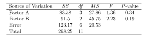
\(\begin{aligned}{*{20}{c}}{MSA = \frac{1}{{I - 1}} \cdot SSA = \frac{1}{3} \cdot 83.58 = 27.86}\\{MSB = \frac{1}{{J - 1}} \cdot SSB = \frac{1}{2} \cdot 91.5 = 45.75}\\{MSE = \frac{1}{{(I - 1)(J - 1)}} \cdot SSE = \frac{1}{6} \cdot 123.17 = 20.53.}\end{aligned}\)
The value of test statistics are
\(\begin{aligned}{*{20}{c}}{{f_A} = \frac{{MSA}}{{MSE}} = \frac{{27.86}}{{20.53}} = 1.36}\\{{f_B} = \frac{{MSB}}{{MSE}} = \frac{{45.75}}{{20.53}} = 2.23.}\end{aligned}\)
There are two ways to make conclusion. Using the table in the appendix or compute P value using a software.
value of test statistics PA and PB:
The PA value when testing hypotheses HOA versus HaA is
\({P_A} = P\left( {F > {f_A}} \right) = P(F > 1.36) = 0.34\)
which was computed using software, and random variable F has Fisher's distribution with degrees of freedom\(I - 1 = 3{\rm{\;and\;}}(I - 1)(J - 1) = 6\)because
\({P_A} = 0.34 > 0.05 = \alpha \)
do not reject hypothesis H0A
at given significance level.
The PB value when testing hypotheses HOB versus HaB is
\({P_B} = P\left( {F > {f_B}} \right) = P(F > 2.23) = 0.19\)
which was computed using software, and random variable F has Fisher's distribution with degrees of freedom\(J - 1 = 2{\rm{\;and\;}}(I - 1)(J - 1) = 6.{\rm{ Because\;}}\)
\({P_B} = 0.19 > 0.05 = \alpha \)
do not reject hypothesis H0B
at given significance level.
Step 8: obtained the values from the table:
using the fact that
\({F_{\alpha ,I - 1,(I - 1)(J - 1)}} = {F_{0.05,3,6}} = 4.76,\)
which was obtained from the table in the appendix, and the fact that
\({F_{0.05,3,6}} = 4.76 > 1.36 = {f_A}\)
do not reject hypothesis H0A
at given significance level.
Also, using the fact that
\({F_{\alpha ,J - 1,(I - 1)(J - 1)}} = {F_{0.05,2,6}} = 5.14,\)
which was obtained from the table in the appendix, and the fact that
\({F_{0.05,2,6}} = 5.14 > 2.23 = {f_B}\)
do not reject hypothesis H0B
at given significance level.
Values are estimated:
Finally, the result can be represented in a table
B)-
The estimates can be computed using the sample means; thus, depending on what value is estimated, the formula is given below
\(\begin{aligned}{*{20}{c}}{\hat \mu = {{\bar x}_{..}} = 50.25}\\{{{\hat \alpha }_1} = {{\bar x}_{1.}} - {{\bar x}_{..}} = 54.33 - 50.25 = 4.08}\\{{{\hat \alpha }_2} = {{\bar x}_{2.}} - {{\bar x}_{..}} = 50.67 - 50.25 = 0.42;}\\{{{\hat \alpha }_3} = {{\bar x}_{3.}} - {{\bar x}_{..}} = 47.33 - 50.25 = - 2.92;}\end{aligned}\)
\(\begin{aligned}{*{20}{c}}{{{\hat \alpha }_4} = {{\bar x}_{4.}} - {{\bar x}_{..}} = 48.67 - 50.25 = - 1.58;}\\{{{\hat \beta }_1} = {{\bar x}_{.1}} - {{\bar x}_{..}} = 53.75 - 50.25 = 3.5}\\{{{\hat \beta }_2} = {{\bar x}_{.1}} - {{\bar x}_{..}} = 53.75 - 50.25 = - 3.25;}\\{{{\hat \beta }_3} = {{\bar x}_{.1}} - {{\bar x}_{..}} = 53.75 - 50.25 = - 0.25.}\end{aligned}\)

Over 30 million students worldwide already upgrade their learning with 魅影直播!