÷ÈÓ°Ö±²¥

Given:

Non-high (sorted):\(1.04, 1.15, 1.23, 1.37, 1.43, 1.57, 1.69, 1.71, 1.92, 1.94, 1.98, 2.06, 2.36, 2.49, 2.55, 2.64, 2.72, 2.82\)

High: \(\;1.55,{\rm{ }}2.02,{\rm{ }}2.02,{\rm{ }}2.05,{\rm{ }}2.35,{\rm{ }}2.57,{\rm{ }}2.93,{\rm{ }}2.94,{\rm{ }}2.97\)

NON HIGH

The minimum is\(1.04\).

Since the number of data values is even, the median is the average of the two middle values of the sorted data set:

\(M = {Q_2} = \frac{{19.2 + 19.4}}{2} = 1.93\)

The first quartile is the median of the data values below the median (or at\(25\% \)of the data):

\({Q_1} = 1.43\)

The third quartile is the median of the data values above the median (or at\(75\% \)of the data):

\({Q_3} = 2.49\)

The maximum is \(2.82.\)

HIGH

The minimum is\(1.55.\)

Since the number of data values is odd, the median is the middle value of the sorted data set:

\(M = {Q_2} = 2.35\)

The first quartile is the median of the data values below the median (or at\(25\% \)of the data):

\({Q_1} = \frac{{2.02 + 2.02}}{2} = 2.02\)

The third quartile is the median of the data values above the median (or at\(75\% \)of the data):

\({Q_3} = \frac{{2.93 + 2.94}}{2} = 2.935\)

The maximum is \(2.97\).

BOXPLOT

The whiskers of the boxplot are at the minimum and maximum value. The box starts at the first quartile, ends at the third quartile and has a vertical line at the median.

The first quartile is at \(25\% \)of the sorted data list, the median at \(50\% \)and the third quartile at \(75\% .\)

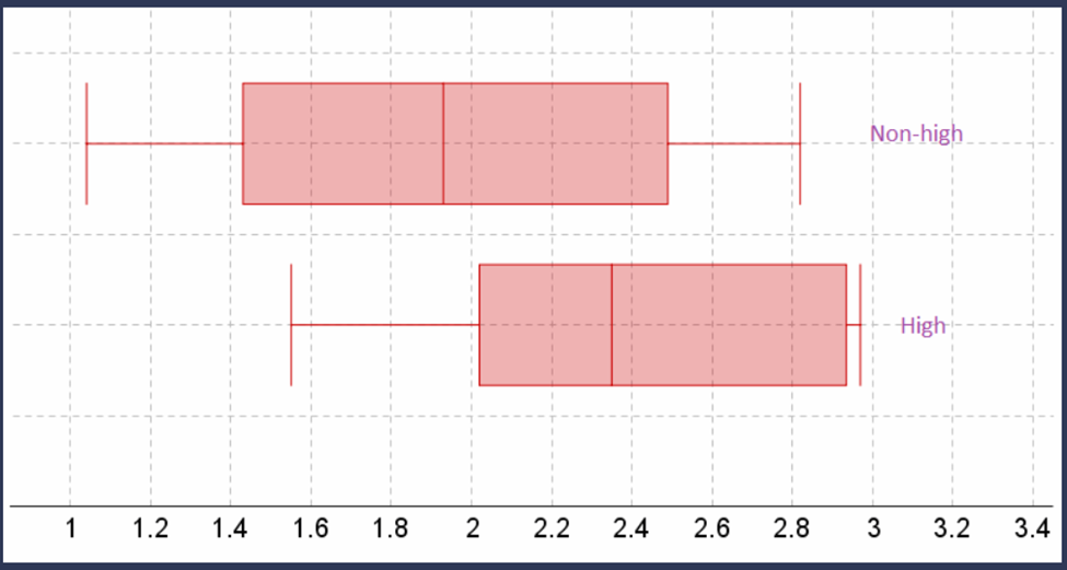
Because the box of the boxplot lies to the right in between the whiskers, the distribution of "High" is severely skewed.

Because the box of the boxplot lies nearly in the middle between the whiskers and the vertical line of the median in the box of the boxplot lies roughly in the middle of the box of the boxplot, the distribution of "Non-high" is roughly symmetric.

Given:

Non-high (sorted):\(1.04,1.15,1.23,1.37,1.43,1.57,1.69,1.71,1.92,1.94,1.98,2.06,2.36,2.49,2.55,2.64,2.72,2.82\)

High: \(1.55,2.02,2.02,2.05,2.35,2.57,2.93,2.94,2.97\)

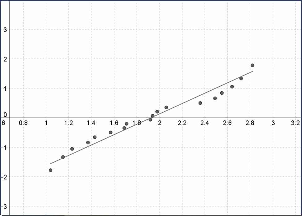
If we want to perform a two-sample\(t\)test, then we require that both sampling distributions of the sample mean are approximately normal.

NON HIGH

We will create a normal probability plot.

The data values are on the horizontal axis and the standardized normal scores are on the vertical axis.

If the data contains \(n\)data values, then the standardized normal scores are the z-scores in the normal probability table of the appendix corresponding to an area of\(\frac{{j - 0.5}}{n}\)(or the closest area) with\(j \in \{ 1,2,3, \ldots .,n\} \).

The smallest standardized score corresponds with the smallest data value, the second smallest standardized score corresponds with the second smallest data value, and so on.

HIGH

We will create a normal probability plot.

The data values are on the horizontal axis and the standardized normal scores are on the vertical axis.

If the data contains\(n\)data values, then the standardized normal scores are the z-scores in the normal probability table of the appendix corresponding to an area of\(\frac{{j - 0.5}}{n}\)(or the closest area) with\(j \in \{ 1,2,3, \ldots ,n\} \).

The smallest standardized score corresponds with the smallest data value, the second smallest standardized score corresponds with the second smallest data value, and so on.

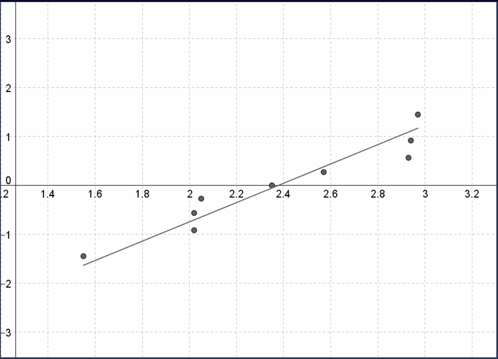
If the pattern in the normal probability plot is roughly linear and does not contain strong The population distribution is approximated normal if the pattern in the normal probability plot is generally linear and does not contain substantial curvature.

Because neither probability map has a lot of curvature and is roughly linear, both population distributions are roughly normal.

The sampling distribution of the sample mean(s) \(\bar x\) is similarly nearly normal since the population distributions are approximately normal. As a result, the two-sample test is suitable.

Given:

\(\begin{array}{l}{n_1} = 18\\{n_2} = 9\\\alpha = 0.01\end{array}\)

The mean is the sum of all values divided by the number of values:

\(\begin{array}{l}{{\bar x}_1} = \frac{{1.04 + 1.15 + 1.23 + \ldots + 2.55 + 2.64 + 2.82}}{{18}} \approx 1.9261\\{{\bar x}_2} = \frac{{1.55 + 2.02 + 2.02 + \ldots + 2.93 + 2.94 + 2.97}}{9} \approx 2.3778\end{array}\)

The variance is the sum of squared deviations from the mean divided by\(n - 1\). The standard deviation is the square root of the variance:

\(\begin{array}{l}{s_1} = \sqrt {\frac{{{{(1.04 - 1.9261)}^2} + \ldots . + {{(2.82 - 1.9261)}^2}}}{{18 - 1}}} \approx 0.5694\\{s_2} = \sqrt {\frac{{{{(1.55 - 2.3778)}^2} + \ldots . + {{(2.97 - 2.3778)}^2}}}{{9 - 1}}} \approx 0.5072\end{array}\)

Given claim: larger the the higher current condition.

The claim is either the null hypothesis or the alternative hypothesis. The null hypothesis and the alternative hypothesis state the opposite of each other. The null hypothesis needs to contain the value mentioned in the claim.

\(\begin{array}{l}{H_0}:{\mu _1} = {\mu _2}\\{H_a}:{\mu _1} < {\mu _2}\end{array}\)

Determine the test statistic:

\(t = \frac{{{{\bar x}_1} - {{\bar x}_2}}}{{\sqrt {\frac{{s_1^2}}{{{n_1}}} + \frac{{s_2^2}}{{{n_2}}}} }} = \frac{{1.9261 - 2.3778}}{{\sqrt {\frac{{{{0.5694}^2}}}{{18}} + \frac{{{{0.5072}^2}}}{9}} }} \approx - 2.093\)

Determine the degrees of freedom (rounded down to the nearest integer):

\(\Delta = \frac{{{{\left( {\frac{{s_1^2}}{{{n_1}}} + \frac{{s_2^2}}{{{n_2}}}} \right)}^2}}}{{\frac{{{{\left( {s_1^2/{n_1}} \right)}^2}}}{{{n_1} - 1}} + \frac{{{{\left( {s_2^2/{n_2}} \right)}^2}}}{{{n_2} - 1}}}} = \frac{{{{\left( {\frac{{{{0.5694}^2}}}{{18}} + \frac{{{{0.5072}^2}}}{9}} \right)}^2}}}{{\frac{{{{\left( {{{0.5694}^2}/18} \right)}^2}}}{{18 - 1}} + \frac{{{{\left( {{{0.5072}^2}/9} \right)}^2}}}{{9 - 1}}}} \approx 17\)

The P-value is the probability of obtaining the value of the test statistic, or a value more extreme. The P-value is the number (or interval) in the column title of Student's T distribution in the appendix containing the t-value in the row\(df = 17\):

\(0.025 < P < 0.05\)

If the P-value is less than or equal to the significance level, then the null hypothesis is rejected:

\(P > 0.01 \Rightarrow {\rm{ Fail to reject }}{H_0}\)

There is not sufficient evidence to support the claim that the true average HAZ depth is larger for the higher current condition than for the lower condition.