/*! This file is auto-generated */ .wp-block-button__link{color:#fff;background-color:#32373c;border-radius:9999px;box-shadow:none;text-decoration:none;padding:calc(.667em + 2px) calc(1.333em + 2px);font-size:1.125em}.wp-block-file__button{background:#32373c;color:#fff;text-decoration:none} Q85E Let \({\rm{X}}\) have a standard... [FREE SOLUTION] | ÷ÈÓ°Ö±²¥

÷ÈÓ°Ö±²¥

Let \({\rm{X}}\) have a standard beta density with parameters \({\rm{\alpha }}\) and \({\rm{\beta }}\).

a. Verify the formula for \({\rm{ E}}\left( {\rm{X}} \right)\) given in the section.

b. Compute \({\rm{E}}\left( {{{\left( {{\rm{1 - X}}} \right)}^{\rm{m}}}} \right){\rm{.}}\) If \({\rm{X}}\) represents the proportion of a substance consisting of a particular ingredient, what is the expected proportion that does not consist of this ingredient?

Short Answer

Expert verified

(a) First use the definition of pdf (that it must integrate to l). From there

\(\frac{{\Gamma ({\rm{\alpha ) \times }}\Gamma ({\rm{\beta }})}}{{\Gamma ({\rm{\alpha + \beta }})}} = \int_{\rm{0}}^{\rm{1}} {{{\rm{x}}^{{\rm{\alpha - 1}}}}} {\rm{ \times (1 - x}}{{\rm{)}}^{{\rm{\beta - 1}}}}{\rm{ \times dx}}\)

Then in the next step use : \(\int_{\rm{0}}^{\rm{1}} {{{\rm{x}}^{\rm{\alpha }}}} {\rm{ \times (1 - x}}{{\rm{)}}^{{\rm{\beta - 1}}}}{\rm{ \times dx}} = \frac{{\Gamma ({\rm{\alpha + 1) \times }}\Gamma {\rm{(\beta )}}}}{{\Gamma ({\rm{\alpha + \beta + 1)}}}}\)

(b)Expected proportion \({\rm{E}}\left( {{{{\rm{(1 - X)}}}^{\rm{m}}}} \right){\rm{ = }}\frac{{\Gamma ({\rm{\alpha + \beta ) \times }}\Gamma ({\rm{\beta + m}})}}{{\Gamma ({\rm{\alpha + \beta + m) \times }}\Gamma {\rm{(\beta )}}}}\)

\({\rm{E((1 - X)) = }}\frac{{\rm{\beta }}}{{{\rm{\alpha + \beta }}}}\)

Step by step solution

01

Definition of Beta density

Where \({\rm{p}}\) and \({\rm{q}}\) are the shape parameters, a and b are the lower and upper bounds of the distribution, respectively, and \({\rm{B(p,q)}}\)is the beta function, the probability density function of the beta distribution has the following general formula: The formula for the beta function is The standard beta distribution is the case where \({\rm{a = 0}}\)and \({\rm{b = 1}}\).

02

Step 2: Verify the formula

(a) The standard beta distribution's pdf is as follows:

\({\rm{f(x,\alpha ,\beta ) = }}\left\{ {\begin{array}{*{20}{l}}{\frac{{\Gamma (\alpha + \beta )}}{{\Gamma {\rm{(\alpha ) \times }}\Gamma (\beta )}}{\rm{ \times }}{{\rm{x}}^{{\rm{\alpha - 1}}}}{\rm{ \times (1 - x}}{{\rm{)}}^{{\rm{\beta - 1}}}}}&{0 \le x \le 1}\\0&{{\rm{ otherwise }}}\end{array}} \right.\)

We start with the definition of pdf (that it must integrate to 1).

\(\begin{aligned}&= \int_0^1 f (x) \times dx \\ &= \int_0^1 {\frac{{\Gamma (\alpha + \beta )}}{{\Gamma (\alpha)\times\Gamma (\beta )}}}\times {x^{\alpha-1}}\times {(1- x)^{\beta- 1}} \times dx\\\frac{{\Gamma (\alpha ) \times \Gamma (\beta )}}{{\Gamma (\alpha + \beta )}} &= \int_0^1 {{x^{\alpha -1}}} \times {(1 - x)^{\beta - 1}} \times dx \\\end{aligned} \)

The standard beta distribution can then be represented as:

\(\begin{aligned}E(X)&= \int_0^1 x\times f(x) \times dx \\ &= \int_0^1 x \cdot \frac{{\Gamma (\alpha + \beta )}}{{\Gamma (\alpha ) \times \Gamma (\beta )}} \times {x^{\alpha - 1}} \times {(1 - x)^{\beta - 1}} \times dx \\&= \frac{{\Gamma (\alpha + \beta )}}{{\Gamma (\alpha ) \times \Gamma (\beta )}} \times \int_0^1 {{x^\alpha }} \times {(1 - x)^{\beta - 1}} \times dx \\\end{aligned}\)

If we substitute this integral with the integral from eqn.l, we will get the same result.

\(\alpha \) by \((\alpha + 1)\) in the eqn.l

\(\begin{aligned}E(X) &= \frac{{\Gamma (\alpha + \beta )}}{{\Gamma (\alpha ) \times \Gamma (\beta )}} \times \frac{{\Gamma (\alpha + 1) \cdot \Gamma (\beta )}}{{\Gamma (\alpha + \beta + 1)}} \\E(X) &= \frac{\alpha }{{\alpha + \beta }} \\\end{aligned}\)

03

 Explain the expected proportion

(b) Similarly, using the given standard beta distribution, \({\rm{E}}\left( {{{{\rm{(1 - X)}}}^{\rm{m}}}} \right)\) can be represented as:

\(\begin{aligned}E\left[{{{(1 - X)}^m}}\right]&= \int_0^1 {{{(1 - x)}^m}}\times f(x)\times dx\\&= \int_0^1 {{{(1 - x)}^m}} \times \frac{{\Gamma (\alpha + \beta )}}{{\Gamma (\alpha ) \times \Gamma (\beta )}} \times {x^{\alpha - 1}} \times {(1 - x)^{\beta - 1}} \times dx \\&= \frac{{\Gamma (\alpha + \beta )}}{{\Gamma (\alpha ) \times \Gamma (\beta )}} \times \int_0^1 {{x^\alpha }} \times {(1 - x)^{\beta + m - 1}} \times dx \\\end{aligned} \)

Now this integral will be same as the integral from (eqn.l) of part(a) if we replace \({\rm{\beta }}\) by \({\rm{(\beta + m)}}\) in the eqn.l

\(\begin{aligned}E\left[ {{{(1 - X)}^m}} \right] &= \frac{{\Gamma (\alpha + \beta )}}{{\Gamma (\alpha ) \times \Gamma (\beta )}} \cdot \frac{{\Gamma (\alpha ) \times \Gamma (\beta + m)}}{{\Gamma (\alpha + \beta + m)}} \hfill \\E\left[ {{{(1 - X)}^m}} \right] &= \frac{{\Gamma (\alpha + \beta ) \times \Gamma (\beta + m)}}{{\Gamma (\alpha + \beta + m) \times \Gamma (\beta )}} \hfill \\\end{aligned} \)

Because \({\rm{X}}\)denotes the proportion of a material that contains a specific ingredient, \({\rm{(1 - X)}}\)denotes the fraction that does not include that ingredient. By substituting \({\rm{m = 1}}\) in the last equation, the expected value may be calculated:

\(\begin{aligned}{l}{\rm{E((1 - X))}} &= \frac{{\Gamma ({\rm{\alpha + \beta ) \times }}\Gamma ({\rm{\beta }} + 1)}}{{\Gamma ({\rm{\alpha + \beta + 1) \times }}\Gamma ({\rm{\beta )}}}}\\{\rm{E((1 - X))}} &= \frac{{\rm{\beta }}}{{{\rm{\alpha + \beta }}}}\end{aligned}\)

Unlock Step-by-Step Solutions & Ace Your Exams!

  • Full Textbook Solutions

    Get detailed explanations and key concepts

  • Unlimited Al creation

    Al flashcards, explanations, exams and more...

  • Ads-free access

    To over 500 millions flashcards

  • Money-back guarantee

    We refund you if you fail your exam.

Over 30 million students worldwide already upgrade their learning with ÷ÈÓ°Ö±²¥!

One App. One Place for Learning.

All the tools & learning materials you need for study success - in one app.

Get started for free

Most popular questions from this chapter

Let X denote the time to failure (in years) of a certain hydraulic component. Suppose the pdf of X is \({\bf{f}}\left( {\bf{x}} \right) = {\bf{32}}/{\left( {{\bf{x}} + {\bf{4}}} \right)^{\bf{3}}}{\rm{ }}{\bf{for}}{\rm{ }}{\bf{x}} < {\bf{0}}\). a. Verify that f (x) is a legitimate pdf. b. Determine the cdf. c. Use the result of part (b) to calculate the probability that the time to failure is between \({\bf{2}}{\rm{ }}{\bf{and}}{\rm{ }}{\bf{5}}\)years. d. What is the expected time to failure? e. If the component has a salvage value equal to \({\bf{100}}/\left( {{\bf{4}} + {\bf{x}}} \right)\)when it is time to fail is x, what is the expected salvage value?

The temperature reading from a thermocouple placed in a constant-temperature medium is normally distributed with mean m, the actual temperature of the medium, and standard deviation. What would the value of s have to be to ensure that \(95\% \)of all readings are within \(.18\)of \(\mu \)?

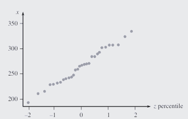
The accompanying normal probability plot was constructed from a sample of \({\rm{30}}\) readings on tension for mesh screens behind the surface of video display tubes used in computer monitors. Does it appear plausible that the tension distribution is normal?

The reaction time (in seconds) to a certain stimulus is a continuous random variable with pdf

\(f(x)= \left\{ {\begin{array}{*{20}{c}}{\frac{3}{2} \times \frac{1}{{{x^2}}}}&{1£x£3} \\0&{{\text{ }}otherwise{\text{ }}}\end{array}} \right.\)

a. Obtain the cdf.

b. What is the probability that reaction time is at most\({\rm{2}}{\rm{.5sec}}\)? Between \({\rm{1}}{\rm{.5}}\) and\({\rm{2}}{\rm{.5sec}}\)?

c. Compute the expected reaction time.

d. Compute the standard deviation of reaction time.

e. If an individual takes more than \({\rm{1}}{\rm{.5sec}}\) to react, a light comes on and stays on either until one further second has elapsed or until the person reacts (whichever happens first). Determine the expected amount of time that the light remains lit. (Hint: Let \({\rm{h(X) = }}\) the time that the light is on as a function of reaction time\({\rm{X}}\).)

The article "The Load-Life Relationship for M50 Bearings with Silicon Nitride Ceramic Balls" (Lubrication Engr., \({\rm{1984: 153 - 159}}\)) reports the accompanying data on bearing load life (million revs.) for bearings tested at a \({\rm{6}}{\rm{.45kN}}\) load.

\(\begin{array}{*{20}{c}}{{\rm{47}}{\rm{.1}}}&{{\rm{68}}{\rm{.1}}}&{{\rm{68}}{\rm{.1}}}&{{\rm{90}}{\rm{.8}}}&{{\rm{103}}{\rm{.6}}}&{{\rm{106}}{\rm{.0}}}&{{\rm{115}}{\rm{.0}}}\\{{\rm{126}}{\rm{.0}}}&{{\rm{146}}{\rm{.6}}}&{{\rm{229}}{\rm{.0}}}&{{\rm{240}}{\rm{.0}}}&{{\rm{240}}{\rm{.0}}}&{{\rm{278}}{\rm{.0}}}&{{\rm{278}}{\rm{.0}}}\\{{\rm{289}}{\rm{.0}}}&{{\rm{289}}{\rm{.0}}}&{{\rm{367}}{\rm{.0}}}&{{\rm{385}}{\rm{.9}}}&{{\rm{392}}{\rm{.0}}}&{{\rm{505}}{\rm{.0}}}&{}\end{array}\)

a. Construct a normal probability plot. Is normality plausible?

b. Construct a Weibull probability plot. Is the Weibull distribution family plausible?

See all solutions

Recommended explanations on Math Textbooks

View all explanations

What do you think about this solution?

We value your feedback to improve our textbook solutions.

Study anywhere. Anytime. Across all devices.