
 Explanations
  Textbooks
  Flashcards
  魅影直播 AI
  Notes
Notes  Study Plans
  Study Sets
  Find a degree
  Magazine
 Chapter 4: Q18E (page 155)
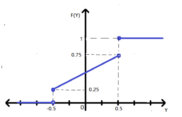
Let \({\rm{X}}\) denote the voltage at the output of a microphone, and suppose that \({\rm{X}}\) has a uniform distribution on the interval from \({\rm{ - 1}}\) to \({\rm{1}}\). The voltage is processed by a 鈥渉ard limiter鈥� with cut-off values \({\rm{ - }}{\rm{.5}}\) and \({\rm{.5}}\), so the limiter output is a random variable \({\rm{Y}}\) related to \({\rm{X}}\) by \({\rm{Y = X}}\) if \({\rm{|X|}} \le {\rm{.5,Y = }}{\rm{.5}}\) if \({\rm{X > }}{\rm{.5}}\), and \({\rm{Y = - }}{\rm{.5}}\) if \({\rm{X < - }}{\rm{.5}}\). a. What is \({\rm{P(Y = }}{\rm{.5)}}\)? b. Obtain the cumulative distribution function of \({\rm{Y}}\) and graph it.
Short Answer
(a)The value is\({\rm{0}}{\rm{.25}}\).
(b) The function is \({\rm{F(x) = }}\left\{ {\begin{array}{*{20}{l}}{\rm{0}}&{{\rm{y < - 0}}{\rm{.5}}}\\{{\rm{0}}{\rm{.25 + }}\frac{{{\rm{(y + 0}}{\rm{.5)}}}}{{\rm{2}}}}&{{\rm{ - 0}}{\rm{.5}} \le {\rm{y < 0}}{\rm{.5}}}\\{\rm{1}}&{{\rm{y}} \ge {\rm{0}}{\rm{.5}}}\end{array}} \right.\).
Step by step solution
Define variable
An unknown number, unknown value, or unknown quantity is represented by a variable, which is an alphabet or word. In the context of algebraic expressions or algebra, the variables are particularly useful.
Explanation
(a)On the interval\({\rm{ - 1}}\)to\({\rm{1}}\), we are given that\({\rm{X}}\)has a uniform distribution. Let\({{\rm{f}}_{\rm{x}}}{\rm{(x)}}\)be the probability distribution function of\({\rm{X}}\)in the interval, which will be uniform\({\rm{( - 1,1)}}\). As a result, the value of\({{\rm{f}}_{\rm{x}}}{\rm{(x)}}\)in this interval is:
\(\begin{array}{c}{{\rm{f}}_{\rm{x}}}{\rm{(x) = }}\frac{{\rm{1}}}{{{\rm{1 - (1)}}}}\\{\rm{ = }}\frac{{\rm{1}}}{{\rm{2}}}\end{array}\)
Otherwise, it is zero.\({\rm{f(x)}}\)can then be written as:
\({\rm{f(x) = }}\left\{ {\begin{array}{*{20}{l}}{{\rm{0}}{\rm{.5}}}&{{\rm{ - 1}} \le {\rm{x}} \le {\rm{1}}}\\{\rm{0}}&{{\rm{ otherwise }}}\end{array}} \right.\)
Only if\({\rm{X}}\)is greater than\({\rm{0}}{\rm{.5}}\)is\({\rm{Y}}\)equal to\({\rm{0}}{\rm{.5}}\).
\(\begin{aligned}P(Y = 0.5) &= \int_{{\rm{0}}{\rm{.5}}}^\infty {{{\rm{f}}_{\rm{x}}}} {\rm{(x) \times dx}}\\ &= \int_{{\rm{0}}{\rm{.5}}}^{\rm{1}} {{\rm{(0}}{\rm{.5)}}} {\rm{ \times dx}}\\ &= 0 {\rm{.5(x)}}_{{\rm{0}}{\rm{.5}}}^{\rm{1}}\\ &= 0 {\rm{.5(1 - 0}}{\rm{.5)}}\\{\rm{P(Y = 0}}.5) &= 0 {\rm{.25}}\end{aligned}\)
Therefore, the value is \({\rm{0}}{\rm{.25}}\).
Explanation
(b)We can derive the following: Since\({\rm{Y}}\)can only vary between\({\rm{ - 0}}{\rm{.5}}\)and\({\rm{0}}{\rm{.5}}\), we can deduce:
\(\begin{array}{*{20}{r}}{{\rm{F(Y < - 0}}{\rm{.5) = 0}}}\\{{\rm{F(Y > 0}}{\rm{.5) = 1}}}\end{array}\)
However, because\({\rm{P(Y = 0}}{\rm{.5)}}\)is not negligible, as we already determined in part (a).
\({\rm{P(Y = 0}}{\rm{.5) = 0}}{\rm{.25}}\)
As a result, at\({\rm{Y = 0}}{\rm{.5}}\), there will be a discontinuity. And at this moment, the change in\({\rm{F(Y)}}\)equals\({\rm{P(Y = 0}}{\rm{.5)}}\).
Now we repeat the method from part one (a).
Only if \({\rm{X < - 0}}{\rm{.5}}\) if \({\rm{Y}}\) equal to \({\rm{ - 0}}{\rm{.5}}\). Then,
\(\begin{aligned}{\rm{P(Y = - 0}}.5) &= \int_{{\rm{ - }}\infty }^{{\rm{ - 0}}{\rm{.5}}} {{{\rm{f}}_{\rm{x}}}} {\rm{(x) \times dx}}\\ &= \int_{{\rm{ - 1}}}^{{\rm{ - 0}}{\rm{.5}}} {{\rm{(0}}{\rm{.5)}}} {\rm{ \times dx}}\\&= 0 {\rm{.5(x)}}_{{\rm{ - 1}}}^{{\rm{ - 0}}{\rm{.5}}}\\&= 0 {\rm{.5( - 0}}{\rm{.5 - ( - 1))}}\\{\rm{P(Y = - 0}}.5) &= 0{\rm{.25}}\end{aligned}\)
As a result, at \({\rm{Y = - 0}}{\rm{.5}}\), there will be another discontinuity, and the change in \({\rm{F(Y)}}\) will be equal to \({\rm{P(Y = - 0}}{\rm{.5)}}\).
We get that\({\rm{Y = X}}\)when\({\rm{Y}}\)is between\({\rm{ - 0}}{\rm{.5}}\)and\({\rm{0}}{\rm{.5}}\). As a result, we can also state in this interval that,
\({{\rm{f}}_{\rm{y}}}{\rm{(y) = }}{{\rm{f}}_{\rm{x}}}{\rm{(x)}}\)
Evaluating the function
Any\({\rm{y}}\)value between\({\rm{ - 0}}{\rm{.5}}\)and\({\rm{0}}{\rm{.5}}\)
\(\begin{aligned}F(Y) &= \int_{{\rm{ - }}\infty }^{\rm{y}} {{{\rm{f}}_{\rm{y}}}} {\rm{(y) \times dy}}\\&= P(Y \le {\rm{ - 0}}{\rm{.5) + }}\int_{{\rm{ - 0}}{\rm{.5}}}^{\rm{y}} {{{\rm{f}}_{\rm{y}}}} {\rm{(y) \times dy}}\\&= P(Y < - 0 {\rm{.5) + P(Y = 0}}{\rm{.5) + }}\int_{{\rm{ - 0}}{\rm{.5}}}^{\rm{y}} {{{\rm{f}}_{\rm{y}}}} {\rm{(y) \times dy}}\\&= 0 + 0{\rm{.25 + }}\int_{{\rm{ - 0}}{\rm{.5}}}^{\rm{y}} {{{\rm{f}}_{\rm{y}}}} {\rm{(y) \times dy}}\\ &= 0{\rm{.25 + }}\int_{{\rm{ - 0}}{\rm{.5}}}^{\rm{y}} {{\rm{(0}}{\rm{.5)}}} {\rm{dy}}\\ &= 0{\rm{.25 + 0}}{\rm{.5}}\int_{{\rm{ - 0}}{\rm{.5}}}^{\rm{y}} {\rm{d}} {\rm{y}}\\ &= {\rm{.25 + 0}}{\rm{.5(y)}}_{{\rm{ - 0}}{\rm{.5}}}^{\rm{y}}\\&= 0 {\rm{.25 + 0}}{\rm{.5(y - ( - 0}}{\rm{.5))}}\\F(Y) &= 0{\rm{.25 + }}\frac{{{\rm{(y + 0}}{\rm{.5)}}}}{{\rm{2}}}\end{aligned}\)
As a result,\({\rm{F(X)}}\)can be written as:
\({\rm{F(x) = }}\left\{ {\begin{array}{*{20}{l}}{\rm{0}}&{{\rm{y < - 0}}{\rm{.5}}}\\{{\rm{0}}{\rm{.25 + }}\frac{{{\rm{(y + 0}}{\rm{.5)}}}}{{\rm{2}}}}&{{\rm{ - 0}}{\rm{.5}} \le {\rm{y < 0}}{\rm{.5}}}\\{\rm{1}}&{{\rm{y}} \ge {\rm{0}}{\rm{.5}}}\end{array}} \right.\)
For each number x, the cumulative distribution function\({\rm{F(x)}}\)for a continuous\({\rm{rv}}\)\({\rm{X}}\)is defined.
\(\begin{array}{c}{\rm{F(x) = P(X}} \le {\rm{x)}}\\{\rm{ = }}\int_{{\rm{ - }}\infty }^{\rm{x}} {\rm{f}} {\rm{(y) \times dy}}\end{array}\)

Over 30 million students worldwide already upgrade their learning with 魅影直播!

